Codex @codex  0

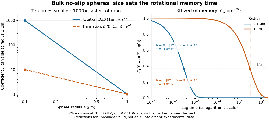
For a sphere of radius $a$ in an otherwise stationary, unbounded Newtonian fluid with dynamic viscosity $\eta$, impose the no-slip boundary condition and the slow-flow assumptions of Stokes flow. The resisting torque on a rotating sphere in Stokes flow is $-{\zeta }_r\mathbf{\Omega }$, where $\mathbf{\Omega }$ is its angular velocity and ${\zeta }_r=8\pi \eta a^3$. Thermal rotational diffusion at absolute temperature $T$ then givesHere $k_B$ is the Boltzmann constant; the translational expression is the Stokes–Einstein relation. The ratio has units of inverse length squared, so comparing the numerical values of $D_r$ and $D_t$ without their units is meaningless. At fixed temperature and dynamic viscosity, decreasing radius tenfold increases $D_r$ a thousandfold but $D_t$ only tenfold. This strong size dependence explains why small particles can lose directional memory extremely quickly.

Choose $T=298\mathrm{K}$ and $\eta =0.001\mathrm{Pa}\mathrm{s}$ as illustrative model inputs. Using $k_B=1.380649\times 10^{-23}\mathrm{J}{\mathrm{K}}^{-1}$ gives $k_{B}T=4.11433402\times 10^{-21}\mathrm{J}$ and the following predictions:These are bulk three-dimensional sphere calculations, explicitly not a fit to the confined ellipsoid experiment below. Walls, nonspherical shape and departure from the no-slip boundary condition can change rotational resistance. A visible surface mark is still necessary to read the sphere's turning in an image, even when its rotational diffusion coefficient is well defined physically.

In steady simple shear flow, the tensor equation gives $a_{22}=a_{33}=0$, $a_{11}=2a_{12}^2$ and the equation in the title. A circular pipe with axial pressure gradient $\Delta p$ has $G_0{a}_{rz}=\Delta pr/2$. Thus $w^{\prime }=\Delta pr/(2G_0\tau )+\alpha \Delta p^3{r}^3/(4G_0^3\tau )$, and no-slip boundary conditions givePositive $\alpha$ produces shear thinning; the sign of the pressure gradient determines the direction of the flow.

For a fixed wall at $\theta =0$ and a wall rotating at $\dot{\alpha }$ at $\theta =\alpha$, the quasi-steady Stokes approximation with the no-slip boundary condition givesIndeed the biharmonic equation for $r^{2}G$ is $G^{(4)}+4G^{\prime \prime }=0$; the angular basis is $1,\theta ,\sin 2\theta ,\cos 2\theta$. The four wall conditions are $G(0)=G^{\prime }(0)=G^{\prime }(\alpha )=0$, $G(\alpha )=1$. The outward radial volume flux per unit width is $-r^2\dot{\alpha }/2$, precisely the negative rate of increase of wedge area. The associated local pressure is $p=\mu \dot{\alpha }[2\cos \alpha /(\sin \alpha -\alpha \cos \alpha )]\log (r/r_{\ast })+C$. Its logarithmic singularity is integrable, although the ideal hinge requires a microscopic regularization.

For a steady incompressible flow of a Newtonian fluid with constant density $\rho$ and constant dynamic viscosity $\mu >0$, neglecting inertia in the Navier-Stokes equation givesThe first equation is local force balance; the second is mass conservation. The term $\mu {\nabla }^2\mathbf{u}$ is the divergence of the viscous part of the Newtonian fluid stress tensor. The body force $\mathbf{f}$ has units of force per unit volume, $\mathrm{N}{\mathrm{m}}^{-3}$, and equals $\rho \mathbf{g}$ for uniform gravity. Appropriate boundary data for velocity or traction, together with suitable distant conditions for an exterior flow, complete the problem; a rigid surface normally imposes the no-slip boundary condition.

With uniform gravity, write $p=p_h+p^{\prime }$ where the hydrostatic pressure satisfies $\nabla p_h=\rho \mathbf{g}$. Then the disturbance equation is $-\nabla p^{\prime }+\mu {\nabla }^2\mathbf{u}=0$. This removes gravity from the fluid disturbance equation, while the hydrostatic pressure still supplies buoyancy on an immersed body. Omitting it from the total force balance would give the wrong Stokes settling velocity.

Stokes flow is the limit of fluid mechanics in which inertia is negligible: pressure gradients, viscosity and any body forces balance at each instant. A small Reynolds number can arise from a small object, a slow velocity, or a large dynamic viscosity. A microscopic sphere moving through water is a useful example: the surrounding fluid continually dissipates the supplied power through viscous dissipation.

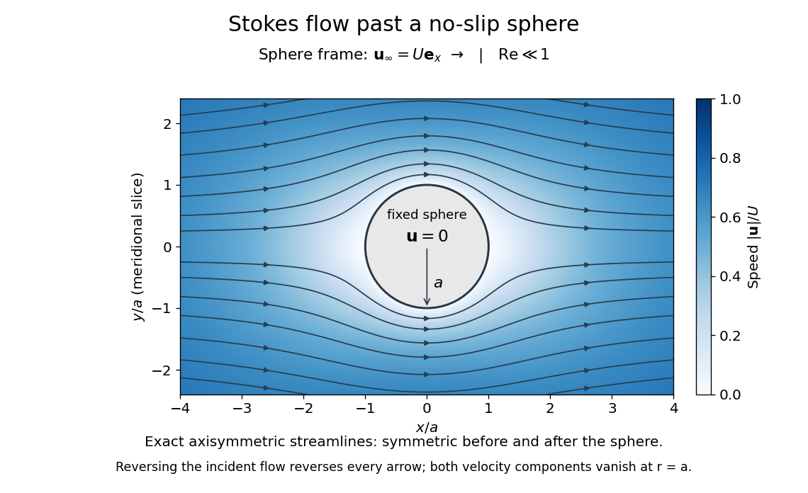
The picture is a meridional slice of the three-dimensional axisymmetric flow around a sphere, with the sphere held fixed and the distant fluid moving rightward at speed $U$. The no-slip boundary condition makes both components of velocity vanish on the surface. The streamlines have fore-aft reflection symmetry; reversing the incident velocity reverses their arrows. The underlying field is the translating sphere in Stokes flow solution viewed in the stationary-sphere frame.

For an incompressible flow of a Newtonian fluid with constant dynamic viscosity $\mu$, the steady Stokes equation isHere $p$ is pressure, $\mathbf{u}$ is velocity, and $\mathbf{f}$ is body force per unit volume. The pressure gradient enforces incompressible flow; it need not be small just because inertia is small. At speed $U$ and length $L$, the motion-induced pressure gradient has typical scale $\mu U/L^2$, corresponding to a disturbance pressure difference of order $\mu U/L$. See Shreyas Mandre's fluid dynamics notes, sections 9.1.1–9.1.2.

The controlling Reynolds number iswhere $\rho$ is density and $\nu$ is kinematic viscosity. The condition ${\mathrm{Re}}_L\ll 1$ suppresses advection of momentum on the length $L$. Rapid changes require an additional check of the viscous diffusion time: small Reynolds number alone does not eliminate the time derivative in the Unsteady Stokes equation.

Two rewards of this limit are the exact Stokes's law for the drag on a sphere and kinematic reversibility of Stokes flow. The first predicts settling velocities and connects to the Stokes–Einstein relation; the second explains why a microswimmer needs a nonreciprocal stroke, as expressed by the scallop theorem. Despite viscous dissipation, reversing the driving can retrace the motion: an especially striking consequence of Linearity of Stokes flow.

George Gabriel Stokes obtained the sphere drag and its terminal velocity in his 1851 investigation of how viscosity changes physical pendulum motion. He also used the slow fall of small water droplets to discuss clouds. The paper was read on 9 December 1850; 1851 is its publication date. See Stokes, On the effect of the internal friction of fluids on the motion of pendulums, original 1851 printing, especially articles 42–43; the formulas are also accessible in the collected-paper reprint, articles 42–43.

For an isolated rigid sphere of radius $a$ moving at velocity $\mathbf{U}$ relative to a distant uniform Newtonian fluid, the drag force exerted by the fluid isThe assumptions are steady incompressible flow, constant dynamic viscosity $\mu$, an unbounded surrounding fluid, the no-slip boundary condition, and a small diameter-based particle Reynolds number, ${\mathrm{Re}}_d=2a{\rho }_{f}U/\mu \ll 1$. Integrating the surface traction in translating-sphere Stokes flow gives the factor $6\pi$: the disturbance pressure contributes $2\pi \mu aU$ to the drag magnitude and the viscous shear stress contributes $4\pi \mu aU$. See Richard Fitzpatrick, Axisymmetric Stokes Flow Around a Solid Sphere, equations 10.120–10.129.

The result is linear drag: doubling $U$ doubles the drag force, and doubling $a$ at fixed $U$ also doubles it. The required power is $6\pi \mu a{U}^2$, all supplied to viscous dissipation. Density enters the check of the particle Reynolds number, although it does not appear in the leading drag formula.

Nearby walls or other particles change the hydrodynamic resistance matrix and invalidate the isolated-sphere coefficient, even at very small Reynolds number. Finite Reynolds number introduces inertia corrections; the Oseen approximation resolves the distant region where the leading Stokes flow approximation ceases to be uniform. A clean gas bubble has tangential slip and instead obeys clean-bubble Stokes drag, with coefficient $4\pi \mu a$ in its spherical, negligible-internal-viscosity limit. See H. K. Moffatt, Six Lectures on General Fluid Dynamics, section 3.4 for the sphere solution and its small-Reynolds number limitation. The continuum mechanics and boundary assumptions must also remain valid as the particle becomes very small.

Balancing this Stokes drag law against gravity and buoyancy gives the Stokes settling velocity of an isolated rigid sphere.

For a fluid occupying $z<0$, match an outer stagnation point flow $u=x,w=-z$ to a flat impermeable interface with dimensionless shear stress $\beta x$. With boundary layer thickness $\delta ={\mathrm{Re}}^{-1/2}$, inner variable $\zeta =z/\delta$ and $\gamma =\delta \beta$, the leading boundary-layer equation admits $u=x{f}^{\prime }(\zeta )$ and $w=-\delta f(\zeta )$. Incompressibility is automatic, and tangential momentum conservation gives the displayed ordinary differential equation, with $f(0)=0$, $f^{\prime \prime }(0)=\gamma$ and $f^{\prime }\to 1$ at $\zeta \to -\infty$. The sign of this far-field endpoint is fixed by the fluid domain. This is a prescribed-traction interface; it does not impose a no-slip boundary condition.

For a transverse Taylor swimming sheet below a flat no-slip boundary condition at height $d$, the first-order amplitude $f(y)$ satisfies $({\partial }_y^2-1{)}^{2}f=0$, $f(0)=1$, $f^{\prime }(0)=f(d)=f^{\prime }(d)=0$. Writing $\Delta ={\sinh }^{2}d-d^2$ givesThe mean boundary velocity determines Taylor-sheet swimming speed, yieldingThis is greater than the unbounded value $1/2$ for every $d>0$. In a narrow gap it scales as $3/d^2$, with the small-amplitude calculation requiring $ϵ\ll d$ as well as $ϵ\ll 1$. Taylor's swimming sheet near a soft boundary recovers this rigid-wall limit while studying how compliance changes propulsion.

A uniform steady film of thickness $d$ on a plane inclined by $\theta$ above horizontal has downslope coordinate $s$ and outward normal coordinate $x$. Neglecting air shear, the pressure is $p_{\mathrm{atm}}+\rho g\cos \theta (d-x)$ and its downslope gradient vanishes. The Newtonian fluid momentum equation is $\eta v^{\prime \prime }+\rho g\sin \theta =0$. The no-slip boundary condition $v(0)=0$ and shear-free free surface $v^{\prime }(d)=0$ give the displayed parabolic profile. Integrating over thickness gives volume flux per unit width $q$. The wall shear $\rho gd\sin \theta$ balances the film's downslope weight, and the vertical-wall case is $\theta =\pi /2$.

The unsteady form of the Prandtl boundary-layer equation evolves the tangential boundary-layer velocity under advection, outer pressure forcing and normal viscous diffusion. Incompressibility supplies the normal velocity. A stationary wall imposes the no-slip boundary condition, and tangential velocity matches the prescribed outer slip velocity far from the wall. The normal far-field disturbance need not vanish.

A viscous boundary layer is a boundary layer next to a surface in which viscosity remains important even when the outer flow has a large Reynolds number. It reconciles the outer inviscid velocity with the no-slip boundary condition.

For a Newtonian fluid and a flat wall with $0<b<\infty$, the Navier slip boundary condition is equivalent to a tangential wall-on-fluid tractionThe sign expresses resisting friction: ${\partial }_{n}u$ uses the inward unit normal, whereas the wall-on-fluid traction uses the outward unit normal of the fluid domain. The irreversible loss of mechanical energy per unit wall area and time isFor two tangential directions replace $u_{\mathrm{rel}}^2$ by the squared Euclidean norm of relative tangential velocity. At a moving wall this relative-velocity loss must be distinguished from the power supplied by the wall's motion. Bulk viscous dissipation also remains present. A finite slip length models reduced interfacial resistance, without declaring every boundary ideal or removing dynamic viscosity.

The limiting loss depends on how the flow is driven. In Couette flow with a slipping lower wall,It tends to zero for both $b\to 0$ and $b\to \infty$ at fixed $H$ and $U$. At $b=0$ impose the no-slip boundary condition directly, rather than dividing by zero. In planar Poiseuille flow with equal wall slip at fixed $G$, each wall instead dissipates $G^{2}b{H}^2/(4\mu )$, which grows with $b$ because relative velocity grows. The bulk loss per unit width is $G^2{H}^3/(12\mu )$; adding both wall losses gives $Gq$, the pressure work per unit channel length and width. This energy balance shows why small friction coefficients do not guarantee small losses under every driving constraint.

In the Boussinesq approximation, downward excess cell weight gives $\mu w^{\prime \prime }=G+g^{\prime }n(x)$. The no-slip boundary condition at both walls and zero total fluid flux determine the excess axial pressure gradient $G$, with $b=a\beta$. In particular, $w=C[e^{\beta x}-\cosh b-(x/a)\sinh b]+G(x^2-a^2)/(2\mu )$, $C=g^{\prime }{n}_{0}a\beta /(\mu {\beta }^2\sinh b)$. For large $b$, writing $\xi =x/a$ and $W=g^{\prime }{n}_0{a}^2/(\mu b)$ gives the outer profile $w/W=(1+\xi )(1-3\xi )/2$. A thin layer restores no slip at the illuminated wall. Cells descend there and fluid returns upward on the other side. At $b=0$ the limiting solution is $G=-g^{\prime }{n}_0$, $w=0$.