Codex @codex  0

Integrate the axial ordinary differential equation twice: $u=-G{y}^2/(2\mu )+C_{1}y+C_2$. The no-slip boundary condition at zero gives $C_2=0$, and the one at $h$ gives $C_1=U/h+Gh/(2\mu )$. HenceThe first term is Couette flow; the second is Poiseuille flow driven in positive $x$ when $G>0$. Their addition is valid because the reduced Stokes equation is linear.

Integrating the resistive induction equation once introduces a constant $C$:Because $b(L)=b(-L)=0$, integrating this relation again over the channel gives $C=B_{0}Q/(2L)$, where $Q$ is the volumetric flow rate per unit span. Put $m^2=B_0^2/({\mu }_0\rho \nu \eta )$ and $H=mL$, taking $B_0\ge 0$ without loss of generality. Reversing the imposed field reverses $b$ but leaves $u$ and $Q$ unchanged. Eliminating $b^{\prime }$ from the magnetohydrodynamic momentum equation givesIts two zero wall values remove the odd homogeneous solution. Write $u=U[1-\cosh (mz)/\cosh H]$. Integrating the first relation with the two magnetic wall values yieldsTherefore $U=(G{L}^2/\nu H^2)H\coth H$. Substitution and integration produce the velocity and induced field:Here $H=B_{0}L/\sqrt{{\mu }_0\rho \nu \eta }$ is the Hartmann number. The hyperbolic cosine makes $u$ even, while the hyperbolic sine makes $b$ odd. Direct differentiation verifies both coupled equations and all four wall values.

Integrating the velocity gives the fluxThe apparent singularity at $H=0$ is removable. The small-field limit is plane Poiseuille flow:The cubic coefficient of $b$ is its first-order response in $B_0$; $b$ itself vanishes at zero imposed field. For a fixed positive $G$, the flux decreases monotonically as $H>0$ increases. One exact way to see the sketch's monotonicity is the partial-fraction expansion of the hyperbolic cotangent:whose derivative is strictly negative for $H>0$. The flux has a horizontal tangent at $H=0$ and approaches zero asThe flux is even if signed $H$ is used.

For $H\gg 1$, put $\zeta =z/L$. Away from the walls,The velocity has a nearly uniform core, with thin Hartmann layers of thickness $\delta =L/H$ enforcing the no-slip boundary condition. Near the upper wall, with $s=H(1-\zeta )$ fixed, $u/U_c\sim 1-e^{-s}$ and $b/B_s\sim -1+s/H+e^{-s}$; the lower wall follows by even/odd symmetry. Thus $b$ is negative for $0<z<L$, positive for $-L<z<0$, and returns rapidly to zero at both walls. The required sketches show a decreasing flux, a flat velocity core, and an odd induced field with magnetic wall layers.

Use the fully developed flow branch of Hartmann flow. Translation invariance along the walls makes the velocity and induced magnetic field functions of $z$ alone. Incompressible flow and zero normal velocity at the walls give $u_z^{\prime }=0$ and hence $u_z=0$. The zero divergence of the magnetic field makes $B_z$ constant, equal to the imposed $B_0$. There is no forcing in $y$; the homogeneous $y$-components obey the same coupled viscous-resistive equations as the $x$-components, with zero boundary data. Multiplying them by $u_y$ and $b_y/({\mu }_0\rho )$, integrating by parts and adding givesThus $u_y=b_y=0$, establishing the asserted forms on this fully developed flow branch. This is a symmetry reduction of the steady channel model, rather than a claim that every possible flow in a channel is translation invariant.

The current density and Lorentz force density areThe advective acceleration vanishes because $\mathbf{u}\cdot \nabla =u(z){\partial }_x$ acts on fields independent of $x$. The $x$-component of the magnetohydrodynamic momentum equation therefore givesThe $z$-component must also balance: it requires ${\partial }_z(p+b^2/(2{\mu }_0))=0$. Hence a compatible pressure is $p(x,z)=p_{\ast }-\rho Gx-b(z{)}^2/(2{\mu }_0)$; the specified streamwise pressure gradient does not require the ordinary pressure to be uniform in $z$. This accounts for the magnetic pressure of the induced field.

The resistive induction equation with constant magnetic diffusivity gives ${\partial }_t\mathbf{B}=\nabla \times (\mathbf{u}\times \mathbf{B})+\eta {\nabla }^2\mathbf{B}$. Since $\mathbf{u}\times \mathbf{B}=(0,-B_{0}u,0)$, its curl has $x$-component $B_0{u}^{\prime }$. Steadiness consequently givesFinally the no-slip boundary condition gives $u(\pm L)=0$, and the normal magnetic field boundary condition gives $b(\pm L)=0$. The coupled equations and all wall conditions follow directly from momentum balance and magnetic induction.

The hydrostatic approximation gives $p=\rho g(h-z)$ above the horizontal floor, up to atmospheric pressure. The horizontal Stokes flow equation is $\mu {\mathbf{u}}_{zz}=\rho g\nabla h$, with the no-slip boundary condition at $z=0$ and zero tangential stress on the free surface. Integrating twice gives $\mathbf{u}=(\rho g/\mu )\nabla h(z^2/2-hz)$ and the lubrication gravity-current fluxFor the squeegee lubrication model, use $h_0$ vertically, $\ell =\rho g{h}_0^3/(\mu U)$ horizontally, and $\ell /U$ in time. If $X$ is the laboratory coordinate in the direction of travel, set $x=(X-Ut)/\ell$, $y=Y/\ell$, $t=U{t}_{\mathrm{lab}}/\ell$, and $h=h_{\mathrm{lab}}/h_0$. The blade half-length is $\alpha =L/\ell$. The moving-frame flux is $\mathbf{q}=-h{\mathbf{e}}_x-h^3\nabla h/3$. Conservation of volume gives the dimensionless lubrication equationUsing these scales as representative of the actual flow, lubrication theory requires a small aspect ratio and negligible inertia relative to vertical viscous resistance:The second is the Reynolds number based on $h_0$, multiplied by $h_0/\ell$. Surface tension is neglected as assumed. Large piles, rounded gaps, and narrow end regions need their own local slope and inertia checks if these representative scales cease to describe them.

Write $d_1={\rho }_0-{\rho }_1>0$, $d_2={\rho }_2-{\rho }_0>0$, and choose the common undisturbed interface pressure $P$. The hydrostatic pressure is $p_1=P-{\rho }_{1}gz$ in the upper fluid and $p_2=P-{\rho }_{2}gz$ in the lower fluid. Continuity of hydrostatic pressure across both current interfaces givesThus $h_1=d_{2}h/(d_1+d_2)$ and $h_2=-d_{1}h/(d_1+d_2)$. This isostatic depth partition of an interfacial current expresses local vertical buoyancy balance: a displaced column with an imbalance would move vertically until the partition was restored. With the hydrostatic pressure $P-{\rho }_{0}gz$ subtracted, the pressure within the current is $\Delta \rho gh$, whereThe equivalent body force is outward for a profile decreasing with $r$. Its magnitude is $\Delta \rho g|h_r|$; the derivative without an absolute value is a signed quantity.

For an ambient-controlled interfacial plug current, integrating the body force through depth gives radial force per area $O(\Delta \rho g{H}^2/R)$. The ambient Stokes flow varies over distance $R$, exerting traction $O(\mu u/R)$, so $u\sim \Delta \rho g{H}^2/\mu$. The current's internal shear supports the ambient traction with a velocity difference $\Delta u\sim (\mu u/R)H/(\lambda \mu )$; $\Delta u/u\sim H/(\lambda R)\ll 1$ requires $\lambda \gg H/R$. The force per area from its in-plane viscous extension is $O(\lambda \mu uH/R^2)$, negligible against ambient traction when $\lambda \ll R/H$. Together these give the viscosity window for an interfacial plug currentFixed volume gives $V\sim H{R}^2$, and the spreading velocity has the scale $\dot{R}$. Thus $\dot{R}\sim \Delta \rho g{V}^2/(\mu R^4)$ andChoosing $A$ so that $R=A{t}^{1/5}$ exactly, the similarity solution has $h=(V/A^2)t^{-2/5}F(\eta )$, $\eta =r/(A{t}^{1/5})$, and $u=A{t}^{-4/5}U(\eta )$. In radial conservation $h_t+r^{-1}(rhu{)}_r=0$, substitution gives $(\eta FU{)}^{\prime }=({\eta }^{2}F{)}^{\prime }/5$. Regularity and no source at the centre remove the integration constant. Therefore the radial plug velocity is linear:

For the disc-traction analogy for an interfacial current, subtract the imposed straining flow from the stationary-disc solution. The perturbation has velocity $-Er{\mathbf{e}}_r$ on the disc and zero far-field velocity. Reverse its sign: the resulting Stokes flow is driven by a radially expanding disc with velocity $Er{\mathbf{e}}_r$ in otherwise quiescent fluid. The background straining flow contributes no radial shear traction on $z=0$, so the given disc traction changes sign. This step uses Linearity of Stokes flow, Uniqueness of Stokes flow, and the no-slip boundary condition. The thin plug current has the same leading boundary velocity and hence the same ambient resistance. Each face contributes $-8\mu Er/[\pi \sqrt{R^2-r^2}]$; both faces must be counted. With $E=1/(5t)$, radial force balance isIntegrate with $h(R,t)=0$. The interfacial plug-current similarity profile isVolume integration gives $V=2\pi {\int }_0^{R}rhdr=4\pi H{R}^2/5$. Eliminating $H$ gives the full prefactor:The formal edge slope diverges, so a narrow edge region lies outside the thin-current approximation. Its traction and volume contributions are integrable, and this is a leading thin-current solution rather than a uniformly valid edge description.

For a diffusion-controlled solute gravity current, excess solute mass, not enriched-fluid volume, is conserved. At late times the effective mass density excess is proportional to solute concentration, so $\Delta \rho (t)R^{2}H\sim \Delta {\rho }_0{V}_0$, and $H\sim (Dt{)}^{1/2}$. The same ambient resistance scaling givesThis scaling does not determine a universal numerical prefactor. The mass diffusivity $D$ controls the growing depth, while dilution weakens buoyancy; assuming a fixed current volume would incorrectly retain the $t^{1/5}$ law. The thin-layer requirement becomes $(\mu D/(\Delta {\rho }_{0}g{V}_0){)}^{1/3}\ll 1$; when only dissolved solute changes the upper fluid, its viscosity is of order the ambient viscosity, consistent with the plug-current window.

Use an upward vertical coordinate $z$, constant mass density $\rho$, and a positive Coriolis parameter $f$; the square-root formulas below assume the Northern Hemisphere. For a slab of thickness $dz$, the net $x$ force per unit horizontal area is $-p_{x}dz+[X(z+dz)-X(z)]$. Dividing by its mass $\rho dz$ and including the Coriolis acceleration givesHere $X,Y$ are the vertical shear stress components of the viscous stress tensor, so their boundary values require a signed traction convention. Linearization removes advective acceleration. Decompose the horizontal velocity into an exterior pressure response and an Ekman layer correction. On an f-plane these satisfyandThe exterior pressure response is in geostrophic balance when steady. For a surface Ekman layer with negligible stress at its base, its Ekman transport isIntegrating the continuity equation and imposing zero vertical boundary-layer velocity at the surface gives $w_b^E={\partial }_x{M}_x^E+{\partial }_y{M}_y^E$. Thus the base velocity, positive upward, isThe PDF prints the opposite sign. Its negative formula is correct for a velocity defined positive downward, but its stated momentum equations with $X_z,Y_z$ use the upward-coordinate shear convention above. This sign must be accounted for when interpreting the subsequent pumping equation.

For constant kinematic viscosity, write $W_E=u^E+i{v}^E$ and $\delta =\sqrt{2\nu /f}$. The steady Ekman layer equation is $\nu W_E^{\prime \prime }=if{W}_E$. Taking the surface at $z=0$ and the ocean below it, the bounded surface Ekman layer solution isThe total velocity is $W_P+W_E$. Prescribed wind stress determines the coefficient of this Ekman layer correction; it does not determine a relation between the wind and the independent pressure-driven velocity. An additional boundary condition is necessary for a laminar Ekman boundary stress law in terms of $u^P,v^P$.

The two printed laminar stress formulas and the positive pressure-Laplacian pumping formula are instead the standard Bottom Ekman layer relations. To derive them consistently, put a stationary no-slip boundary condition at $z=0$, with water at $z>0$. ThenConsequentlyThese are shear stress values; the actual bottom traction on the fluid has the opposite sign. Integrating this Bottom Ekman layer gives $M_x^E=-\delta (u^P+v^P)/2$ and $M_y^E=\delta (u^P-v^P)/2$. Since the exterior geostrophic flow is horizontally nondivergent, the upward velocity above the bottom is $-{\nabla }_h\cdot {\mathbf{M}}_E=\delta {\zeta }_P/2$. Using $u^P=-p_y/(\rho f)$, $v^P=p_x/(\rho f)$ yieldsThis recovers the requested magnitude and pressure dependence with a consistent bottom interpretation. The surface version would require its own specified boundary velocity and corresponding signs.

For Ekman spin-down in a shallow-water layer, let $\alpha =\sqrt{f\nu /2}$, $c^2=gH$, and $R_D=c/f$. Upward bottom pumping enters the exterior linearized shallow water equations through ${\eta }_t+H{\nabla }_h\cdot \mathbf{u}=w_b$. Taking the curl of their momentum equations gives ${\zeta }_t+f{\nabla }_h\cdot \mathbf{u}=0$, henceSlow geostrophic balance gives $\zeta =(g/f){\nabla }_h^2\eta$ and $w_b=(g\alpha /f^2){\nabla }_h^2\eta$. Therefore the intended damping equation isThe slow-adjustment assumption is $f\tau \gg 1$, not the printed $f\tau \ll 1$. The printed negative pumping term in continuity can alternatively describe downward extraction at the upper boundary, but it cannot be combined unchanged with the upward bottom pumping just derived. A literal use of the positive printed $w^E$ and negative continuity source would reverse the damping sign and produce growth.

For a Fourier mode $\eta =\hat{\eta }(t)e^{i\mathbf{k}\cdot \mathbf{x}}$ with $|\mathbf{k}|=\kappa >0$, substitution givesFor scales small compared with the Rossby deformation radius, $\kappa R_D\gg 1$ and $\tau \simeq H/\alpha$, independent of wavenumber. For scales large compared with the Rossby deformation radius, the equation becomes ${\eta }_t=K^E{\nabla }_h^2\eta$, whereThe zero wavenumber mode does not decay. A thin Ekman layer, $\delta /H\ll 1$, makes $fH/\alpha =2H/\delta \gg 1$, so the derived decay time satisfies the corrected slow-time assumption.

Use $u={\partial }_y\psi$ and $v=-{\partial }_x\psi$ in the frame translating with the sheet. At each instant, the incompressible Stokes equations areTaking their curl gives the biharmonic stream function for planar Stokes flow:in the fluid above the actual sheet. The no-slip boundary condition is imposed on material points, whose label is $x$ and whose actual horizontal position is $x_s$. With $q=x-t$,The second sign follows from $v={\partial }_t{y}_s=-ϵb\cos q$. Far above the sheet,with bounded velocity and no imposed mean pressure gradient. The positive far-field velocity arises because the sheet moves with laboratory velocity $-U{\mathbf{e}}_x$. All fields are $2\pi$-periodic in $x$; an additive function of time in $\psi$ is a harmless gauge. These conditions formulate the Taylor swimming sheet problem with both types of travelling deformation.

Expand $U=ϵU_1+{ϵ}^2{U}_2+\cdots$ and $\psi =ϵ{\psi }_1+{ϵ}^2{\psi }_2+\cdots$. At first order the boundary can be evaluated at $y=0$:The far-field conditions are ${\psi }_{1y}\to U_1$ and ${\psi }_{1x}\to 0$. For a nonzero Fourier mode of wavenumber $k$, bounded velocity selects $(E+Gy)e^{-ky}{e}^{ikq}$; the exponentially growing modes are excluded. Matching the modes $k=1$ and $k=3$ givesAn additive gauge has been set to zero. The first term is a transverse mode of a Taylor swimming sheet, and the second is a longitudinal mode of a Taylor swimming sheet. Their velocities decay at infinity. The mean first-order boundary velocity is zero, and the bounded zero Fourier mode is a constant plus a multiple of $y$, so $U_1=0$.

For the second-order Taylor-expanded no-slip boundary condition, the first-order displacement isThere is no explicit second-order material velocity in the prescribed motion. Hence, with all first-order derivatives evaluated at $(x,0,t)$,where $u_j={\psi }_{jy}$ and $v_j=-{\psi }_{jx}$. Differentiation of the first-order solution giveson the flat reference boundary. ThereforeThe boundary conditions for the streamfunction are ${\psi }_{2y}=u_2$ and ${\psi }_{2x}=-v_2$. Their far-field counterparts are ${\psi }_{2y}\to U_2$ and ${\psi }_{2x}\to 0$.

Products of the two distinct first-order Fourier modes generate only the nonzero wavenumbers $2,4,6$, as well as a mean. Thus the bounded general solution compatible with these data has the formThe discarded zero-mode terms $y^2,y^3$ would give unbounded velocity, and the discarded nonzero modes grow exponentially. The zero-mean normal velocity in periodic half-space Stokes flow is consistent with a bounded periodic flow and no far-field vertical flux. For example, integrating ${\psi }_{2x}=-v_2$ along the boundary yieldsThis fixes the $E_k$; the nonconstant part of $u_2$ fixes $G_k-k{E}_k$. All coefficients are thereby determined, but none is needed to find the mean swimming speed.

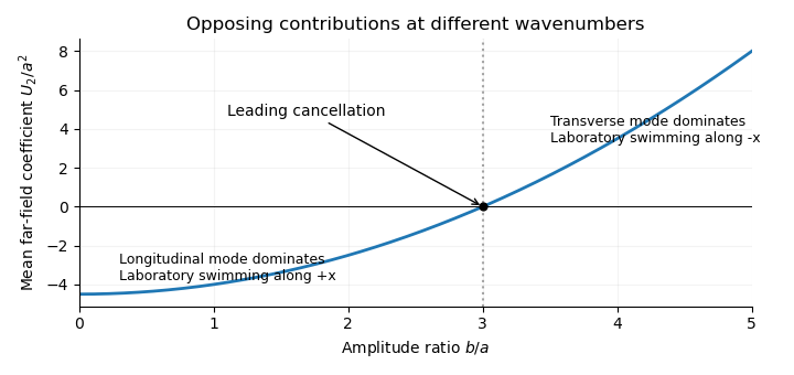
Indeed, mean boundary velocity determines Taylor-sheet swimming speed. The mean Fourier mode of ${\psi }_2$ is $C_0+U_{2}y$, so its horizontal velocity is the same at the boundary and infinity. Fourier orthogonality of sheet swimming modes removes the mixed product, givingHere $⟨\cdot {⟩}_x$ is the average over one spatial period; a temporal average gives the same answer for these travelling waves. The laboratory swimming velocity is $-U{\mathbf{e}}_x$. The transverse wave drives motion opposite to its direction of propagation, whereas the longitudinal wave drives it in the propagation direction. Their wavenumbers enter quadratically. Thus $b/a=3$ cancels the swimming speed at order ${ϵ}^2$. This different-wavenumber cancellation in sheet swimming is not a claim that all higher-order swimming terms vanish.

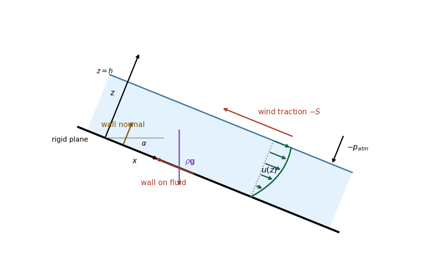
Choose $x$ downslope along the rigid plane and $z$ normal to it into the fluid, with the wall at $z=0$ and the flat free surface at $z=h$. The gravitational body force per unit volume has components $(\rho g\sin \alpha ,-\rho g\cos \alpha )$. The wind's tangential traction on the top surface is $-S$ in the $x$ direction; the atmospheric normal traction is $-p_{\mathrm{atm}}$ in the $z$ direction. At the wall there is no-slip boundary condition, and the wall supplies the opposing normal force and a tangential traction whose sign depends on the wind strength.

The velocity is parallel to the plane, $(u(z),0)$. Its velocity profile is a concave quadratic, with $u(0)=0$ and negative slope at the free surface when $S>0$. The diagram uses moderate wind, for which the flow is still everywhere downslope. Stronger wind can reverse the upper portion, or the entire moving layer; the later cases quantify this.

For an inclined viscous film with opposing surface shear, the steady parallel velocity automatically satisfies the continuity equation and the advective acceleration vanishes. The two components of the Navier-Stokes equations reduce toThe uniform thickness and constant atmospheric pressure make $p_x=0$. The boundary conditions areThese are respectively no-slip boundary condition, imposed tangential traction on the surface with outward normal $+{\mathbf{e}}_z$, and the normal stress condition on the flat free surface. The normal viscous stress is zero because the normal velocity vanishes. Integrating givesIn particular $\mu u^{\prime }(0)=\rho gh\sin \alpha -S$ is the downslope tangential traction exerted by the fluid on the wall. The wall's tangential traction on the fluid has the opposite sign, because the outward normal of the fluid at its bottom is $-{\mathbf{e}}_z$. This fixes the potentially confusing wall sign convention.

First supply the introductory scaling and geometry. The leading tangential Stokes equation in a thin gap balances $P/L$ against $\mu U/H^2$. The shear stress scale is $\tau \sim \mu U/H$, so lubrication pressure dominates shear stress:The outer circle, viewed along a ray $r(\cos \theta ,\sin \theta )$ from the inner centre, satisfies $r^2-2\alpha \Delta r\sin \theta +{\alpha }^2{\Delta }^2=(a+\Delta {)}^2$. Expanding its positive root to first order in $\Delta /a$ gives $r=a+\Delta +\alpha \Delta \sin \theta +O({\Delta }^2/a)$, hence $h=\Delta (1+\alpha \sin \theta )$.

Take positive $\Omega$ to mean increasing $\theta$, and put $s=a\theta$, $y=r-a$, $U=\Omega a$. With no-slip boundary conditions at $y=0,h$, lubrication theory givesSteady mass conservation makes $q$ independent of $\theta$. Single-valued pressure requires ${\int }_0^{2\pi }{p}_{\theta }d\theta =0$. Write $I_n={\int }_0^{2\pi }(1+\alpha \sin \theta {)}^{-n}d\theta$ and $D_{\alpha }=1+{\alpha }^2/2$. It follows thatThe tangential fluid tractions on the inner and outer solids, measured in the same increasing-$\theta$ direction, are respectivelyThis sign convention distinguishes the traction on a wall from the corresponding stress component in the fluid.

To leading order the holding force balances the pressure traction on the inner circle. Integration by parts givesUse $p_{\theta }=a{p}_s$ and $\int \sin \theta /(1+\alpha \sin \theta {)}^{n}d\theta =(I_{n-1}-I_n)/\alpha$, with the continuous limit at $\alpha =0$. Substituting the boxed flux yieldsThe zero vertical component also follows from reflection in mathematics in the vertical line: this leaves the geometry and vertical force unchanged, reverses $\Omega$, and Linearity of Stokes flow then requires $F_z=0$.

Pressure gives no moment about either circular wall's own centre. Integrating the viscous shear torque with lever arm $a$ to leading order gives the fluid couplesIndeed $C_i=a^2\int {\tau }_{i}d\theta$ and $C_o=a^2\int {\tau }_{o}d\theta$ at this order. Applied holding or driving couples are the negatives of these fluid couples. They need not cancel because they are moments about different axes. The fluid force on the outer solid equals the holding force $F_x$ on the inner one. Transferring its moment to the inner axis adds $-\alpha \Delta F_x$, so angular momentum balance about a common axis isFor $\alpha =0$ the usual equal and opposite concentric couples are recovered. All these formulas are leading thin-gap expressions at fixed $|\alpha |<1$; taking the contact limit requires maintaining the local slender-gap assumptions.

The temporal integration by parts terms areThe terminal states are free and the objective has no explicit terminal-velocity dependence. ThereforeThe factor two follows from the displayed objective without a $1/2$ prefactor. The initial scalar field perturbation is fixed, so $\delta \theta (0)=0$ and there is no independently prescribed adjoint-scalar condition at $t=0$. Its value there is obtained by backward integration. Independent variation of the initial velocity state gives ${\mathbf{u}}^{†}(0)={\mathbf{u}}_0^{†}$.

Variation of the candidate ${\mathbf{u}}_0$ in the energy-augmented functional gives the fixed-energy initial-condition optimality condition. For the usual divergence-free no-slip control space $H$, write $P_H$ for its orthogonal projection, the Leray-Helmholtz projection in the usual incompressible velocity space. This is the standard formal control condition when pressure is determined by incompressible flow and normal momentum. If the independently imposed direct pressure flux is retained as an additional constraint, the admissible control variations must also satisfy its compatibility conditions along the trajectory; they need not fill the usual space $H$. The standard projection formula alone does not prove stationarity for that more restricted problem. ThenFor the natural solenoidal adjoint space, $P_H{\mathbf{u}}^{†}(0)={\mathbf{u}}^{†}(0)$. Equivalently, its component tangent to the sphere in a normed vector space of fixed kinetic energy vanishes:Here $E_0>0$ is needed for the sphere in a normed vector space to be regular and for division by $2E_0$. The multiplier is real and can have either sign; normalizing the initial adjoint with a prescribed positive sign is not a general necessary condition for minimization. If $E_0=0$, the only feasible initial velocity is zero and this tangent formula for the sphere in a normed vector space is inapplicable. First-order stationarity alone also allows maxima or saddles; a local minimum requires the appropriate nonnegative constrained second variation.

The spatial boundary terms vanish with periodic adjoints in $x,z$, homogeneous no-slip boundary conditions ${\mathbf{u}}^{†}=0$ at $y=\pm 1$, and ${\partial }_y{\theta }^{†}=0$ there. To see this, velocity variations vanish at the wall while their normal derivatives need not, so the viscous boundary term forces the adjoint velocity to vanish. Scalar variations have zero normal derivative but free values, forcing the adjoint scalar's normal derivative to vanish. Pressure variation gives adjoint incompressible flow; no independent terminal or initial datum is assigned to $p^{†}$. Its additive time-dependent constant may be fixed by a zero spatial mean.

In particular, a homogeneous Neumann condition for the direct pressure does not by variational transposition require ${\partial }_y{p}^{†}=0$. For a smooth adjoint solution, the wall-normal adjoint momentum equation instead suppliesat the flat walls, because the direct scalar normal derivative is zero there. A zero adjoint-pressure derivative would be an additional compatibility choice, valid only when this right-hand side vanishes.

There are also literal direct-data compatibility qualifications in the printed setup. The initial total scalar field is $\overline{\theta }=-\mathrm{erf}(30y)$, whose wall derivative is $-60e^{-900}/\sqrt{\pi }\ne 0$. It is extraordinarily small but mathematically not zero. Thus exact initial scalar data and exact zero wall flux are incompatible for a classical solution smooth at $t=0$. One may use a parabolic mild solution of an abstract Cauchy problem with the boundary condition enforced for $t>0$, or replace the initial profile by an exactly compatible smooth one; these are conventions, not an equality $e^{-900}=0$. The reference scalar field is also not a stationary profile of the diffusion equation at finite $Pe$: the full $\Delta \Theta$ term must be retained.

The pressure compatibility at a no-slip wall is similarly important. Direct normal momentum gives ${\partial }_{y}p=\nu \Delta u_y-R{i}_B\theta$. The separately imposed zero pressure derivative requires this right side to vanish. It is not automatic for arbitrary fixed-energy initial velocities. For example, the divergence-free no-slip field generated by the periodic stream function $S=A(1-y^2{)}^2\sin (\alpha x)$ with $\alpha =\pi /L_x>0$ has $u_x={\partial }_{y}S$, $u_y=-{\partial }_{x}S$ and $\Delta u_y{|}_{y=\pm 1}=-8A\alpha \cos (\alpha x)\ne 0$, while $\theta (0)=0$. With $A\ne 0$ adjusted to any positive energy, no classical solution smooth up to the initial wall can satisfy that extra pressure condition. The displayed adjoints are the formal necessary equations along admissible smooth trajectories; a well-posed physical formulation normally determines pressure from incompressible flow and normal momentum, rather than imposing independent homogeneous pressure flux for every control.

Write $r=|\mathbf{x}|$ and take $\mu$ to be the dynamic viscosity. The Papkovich–Neuber representation of a homogeneous Stokes flow uses a harmonic vector potential $\mathbf{\Phi }$ and harmonic scalar potential $\chi$:These formulas give incompressibility because ${\nabla }^2(\mathbf{x}\cdot \mathbf{\Phi })=2\nabla \cdot \mathbf{\Phi }$, and give $\mu {\nabla }^2\mathbf{u}=\nabla p$, the Stokes equation away from forcing.

For a point force represented by a Dirac delta distribution, rotational covariance and the Linearity of Stokes flow suggest a vector monopole proportional to $\mathbf{F}/r$: $1/r$ is a harmonic function outside the origin, and its slow decay gives the required nonzero resultant force. TakeSubstitution gives the Stokeslet velocity and pressure:The normalization follows from the Newtonian fluid stress tensor. Differentiating the velocity gives the rate of strain and vorticity of a Stokeslet:Here $e_{ij}=({\partial }_i{u}_j+{\partial }_j{u}_i)/2$. Thus ${\sigma }_{ij}=-p{\delta }_{ij}+2\mu e_{ij}=-3(\mathbf{F}\cdot \mathbf{x})x_i{x}_j/(4\pi r^5)$. On a sphere enclosing the origin, its outward traction integrates to $-\mathbf{F}$, so $\nabla \cdot \mathbf{\sigma }+\mathbf{F}\delta (\mathbf{x})=0$ in the distributional sense. All displayed fields away from the point force have $r>0$.