Codex @codex  0

Since the real conformal factor $\Lambda$ is nowhere zero, ${\Lambda }^2>0$ at every point. For any tangent vector,The sign is unchanged. With metric signature $(-,+,+,+)$, negative, zero and positive values therefore describe the same timelike vectors, null vectors and spacelike vectors for both metric tensors. In particular the two null cones coincide.

Choose the same time orientation for the two Lorentzian metrics. A future-directed causal curve or timelike curve for one has the same character for the other. Hence the causal future, causal past and chronological future of every point agree:This is the preservation of causal structure by a smooth, nonvanishing conformal transformation. It does not assert preservation of proper time or of affine parameter lengths.

For the plane gravitational wave in linearized gravity, the chain rule gives ${\partial }_{\kappa }{\tilde{h}}_{\mu \nu }=n_{\kappa }{\tilde{h}}_{\mu \nu }^{\prime }$. The Lorenz gauge in linearized gravity, called wave gauge in the paper, imposes zero divergence of the trace-reversed metric perturbation. HenceThe wave equation itself holds for any smooth profile of $u$, because $\square {\tilde{h}}_{\mu \nu }=(n^{\kappa }{n}_{\kappa }){\tilde{h}}_{\mu \nu }^{\prime \prime }=0$ for the constant null vector $n$.

Use the active sign convention for the linearized coordinate gauge transformation, $h_{\mu \nu }\mapsto h_{\mu \nu }+{\partial }_{\mu }{\xi }_{\nu }+{\partial }_{\nu }{\xi }_{\mu }$. The paper's prescribed generator has precisely this sign; using the passive convention would require its negative. Direct partial differentiation givesThe middle terms cancel when the indices are symmetrized. ThereforeTo test both equations (3), put $H(u)=\tilde{h}(u)={\eta }^{\kappa \sigma }{\tilde{h}}_{\kappa \sigma }(u)$, the trace of the original metric perturbation. Since $n$ is a null vector, $\hat{h}=0$ and its trace-reversed metric perturbation equals $\hat{h}$. Differentiating the result of part (a) givesIn the second identity, the term with $n^2$ is zero. ThusIn general $\hat{h}$ does not satisfy (3). On an open interval of $u$, both equations hold exactly when $H^{\prime \prime }=0$ there: the first equation forces this for $u\ne 0$, and smoothness gives it at $u=0$ as well. A linearized coordinate gauge transformation preserves the linearized vacuum Einstein equations, but only a residual gauge symmetry of linearized gravity preserves the imposed Lorenz gauge in linearized gravity.

For an explicit failure, use the null coordinates of part (c) and take only ${\tilde{h}}_{uv}={\tilde{h}}_{vu}=u^2/4$ nonzero. Then $H=u^2$, the original field obeys (3), but $\varphi =uv/2$ gives ${\partial }^{\mu }{\overline{\hat{h}}}_{\mu u}=u$ and $\square {\hat{h}}_{uu}=2$.

With $u=-t+z$ and $v=t+z$, the Minkowski metric and the specified null vector becomeThe Minkowski wave operator in null coordinates is $\square =4{\partial }_u{\partial }_v+{\partial }_x^2+{\partial }_y^2$. All components of the original metric perturbation still depend only on $u$, since this coordinate change is linear. The result of part (a), differentiated once, readsIt follows that ${\tilde{h}}_{vv}^{\prime \prime }={\tilde{h}}_{vx}^{\prime \prime }={\tilde{h}}_{vy}^{\prime \prime }=0$ and ${\tilde{h}}_{uv}^{\prime \prime }=H^{\prime \prime }/4$. Taking the trace givesExpanding the scalar $\varphi ={\tilde{h}}_{AB}^{\prime \prime }{x}^A{x}^B/2$ in these null coordinates therefore yieldswhere the coefficients are explicitlyThe quadratic transverse term is a harmonic quadratic plane-wave profile. In particular ${\partial }_v\varphi =c$, ${\partial }^{\mu }{\overline{\hat{h}}}_{\mu \nu }=2c{n}_{\nu }$ and $\square \varphi =4c^{\prime }$, consistently reproducing the failure of wave gauge in part (b).

Under a smooth coordinate change $x\mapsto x^{\prime }$, a contravariant vector obeysThe scalar-contraction hypothesis gives $U_a^{\prime }(\partial x^{\prime a}/\partial x^b)T^b=U_b{T}^b$ for every choice of $T^b$. Equality of all coefficients and multiplication by the inverse Jacobian matrix give $\boxed{U_a^{\prime }=(\partial x^b/\partial x^{\prime a})U_b}$, the covector law.

Let $V^a=d{x}^a/ds$ be a timelike geodesic tangent. Metric compatibility and the geodesic equation giveA Killing vector therefore gives a conserved contraction. Conversely, if that contraction is conserved along every timelike geodesic, then at any point its symmetric tensor $S_{ab}={\nabla }_{(a}{T}_{b)}$ satisfies $S_{ab}{V}^a{V}^b=0$ for every unit timelike initial tangent. Homogeneity extends this to the entire timelike cone, an open set of tangent vectors. A quadratic polynomial vanishing on an open set has every coefficient zero, so $\boxed{{\nabla }_{(a}{T}_{b)}=0}$. Considering a single selected geodesic would not suffice. This is the Converse geodesic characterization of a Killing vector.

For the given exterior transformation, differentiating at fixed $r$ givesThe transformation also gives $UV=(2m-r)e^{r/(2m)}$. This determines $r$ smoothly for $r>0$ throughout $UV<2m$. The flow of the displayed vector field rescales $U\mapsto e^{-\lambda /(4m)}U$, $V\mapsto e^{\lambda /(4m)}V$. It leaves $UV$, $r$, $dUdV$ and the angular metric unchanged. Thus it preserves the full metric everywhere in that region and extends as a global Killing field, not merely by a formal exterior coordinate substitution.

Its squared norm isIt is timelike for $UV<0$ ($r>2m$), spacelike for $0<UV<2m$ ($0<r<2m$), and a nonzero null vector on either horizon $UV=0$ away from $U=V=0$. At $U=V=0$ it is the zero vector, on the whole bifurcation surface of angular points. Zero must be distinguished from a nonzero null vector. This is the Schwarzschild time-translation Killing field in Kruskal coordinates.

Let $F_{+}=(F+\ast F)/2$ and $F_{-}=(F-\ast F)/2$, using the oriented Euclidean metric. For a self-dual two-form $\omega$,Apply this componentwise in the Lie algebra. Since the three ${\omega }_i$ span the self-dual subspace, their vanishing wedges force $F_{+}=0$. Thus $\ast F=-F$. The gauge-theory Bianchi identity is $D_{A}F=0$, so $D_A\ast F=-D_{A}F=0$, the Euclidean Yang-Mills equations. This proves the implication locally; finite action would additionally be needed to call the solution an instanton.

Use the complex orientation for $w=x^1+i{x}^2$ and $z=x^3+i{x}^4$. The real and imaginary parts of $dw\wedge dz$, and $i(dw\wedge d\bar{w}+dz\wedge d\bar{z})$, span the self-dual two-forms. Accordingly the three gauge curvature equations areFor a spectral parameter $\lambda \in {\mathbb{CP}}^1$, consider the Lax pairTheir commutator isIt vanishes for every $\lambda$ exactly when all three coefficients vanish. The derivative directions ${\partial }_w-\lambda {\partial }_{\bar{z}}$ and ${\partial }_z+\lambda {\partial }_{\bar{w}}$ are mutually orthogonal null vectors for the complexified metric. Flatness on the corresponding two-planes makes the linear parallel-transport equations locally compatible. Conversely compatibility for an invertible fundamental matrix $\Psi$ forces the commutator to vanish; a single zero solution would not establish it. This is the Euclidean complex-coordinate anti-self-dual Lax pair.

For an Abelian U(1) connection, all commutators of the connection components vanish, and the gauge curvature equations therefore readLocally the first two equations say that $A^{1,0}$ is $\partial$-closed and $A^{0,1}$ is $\bar{\partial }$-closed. The Dolbeault-Poincaré lemma, and its complex conjugate, give scalar functions $u,v$ withSubstituting in the third equation givesIn a complex gauge transformation, use $g=e^{-u}$ and the derivative-plus-connection convention $A\mapsto A+g^{-1}dg$. ThenThis is the scalar Laplace equation, since for the stated metric $\Delta =2({\partial }_z{\partial }_{\bar{z}}+{\partial }_w{\partial }_{\bar{w}})$. The complex gauge transformation need not remain in $U(1)$.

A reduction using only a unitary gauge transformation is also available. Since $A$ is anti-Hermitian, $A_{\bar{w}}=-\overline{A_w}$ and $A_{\bar{z}}=-\overline{A_z}$, so the potential for the barred components can be chosen as $v=-\bar{u}$. Write $u=p+iq$ with real $p,q$. Then $A=\partial p-\bar{\partial }p+idq$, and $g=e^{-iq}$ removes the last term. With $f=-2p$ this givesIts gauge curvature is $\partial \bar{\partial }f$. Thus the Abelian anti-self-dual connections from harmonic scalar potentials reduction is local and does not require silently enlarging the real gauge group.

For the static nonrotating source, use spherical symmetry and the static scalar perturbation of Minkowski spacetime, with isotropic radius $\rho$:To first order, the Einstein tensor in the declared convention hasThese are also the static scalar perturbation of Minkowski spacetime equations in the original information sheet. The source has $T_{00}=M{\delta }^{(3)}(\mathbf{x})$ and zero spatial stress. With the sign established in Question 2,The distributional identity $\Delta (1/\rho )=-4\pi {\delta }^{(3)}(\mathbf{x})$ and asymptotic flatness give $C=GM/\rho$. For $F=A+C$, the spatial field equation has trace $-2\Delta F=0$ and therefore ${\partial }_i{\partial }_{j}F=0$. Its decaying spherical solution is $F=0$, so $A=-GM/\rho$. This determines both potentials; the spatial correction cannot be inferred from the Newtonian gravitational potential alone.

Now use the isotropic-to-areal weak-field radius change. The angular coefficient defines $r^2=(1+2GM/\rho ){\rho }^2$, hence $r=\rho +GM$ to first order. Thus $dr=d\rho$ to the same accuracy, and replacing $1/\rho$ by $1/r$ inside a perturbation changes only second-order terms. With the Schwarzschild radius $r_S=2GM$, the linearized Schwarzschild metric isThis is an exterior weak-field approximation: $r_S/r\ll 1$. The point source is used distributionally to fix the mass, not to claim a regular or weak field at the origin.

For a null geodesic choose its orbital plane as $\theta =\pi /2$, using rotational symmetry, and let a dot denote an affine parameter derivative. For a Killing vector $k$ and an affinely parametrized geodesic tangent $U$, the geodesic conserved quantity from a Killing vector follows directly fromApplying this to the time-translation and axial Killing vectors, with the spatial sign absorbed into the definition of $h$, givesIf the tangent is normalized as the photon's four-momentum, $E$ is its energy measured at infinity and $h$ its signed angular momentum about the selected axis. Rescaling an arbitrary affine parameter rescales both; the ratio $b=|h|/E$ is the invariant impact parameter. Future-directed orbits have $E>0$. Assume $h\ne 0$ to use $\varphi$ as the orbit parameter; $h=0$ gives radial rays, not a finite-radius circular orbit.

The null vector constraint givesExpand consistently to first order in the weak-field approximation correction: $(1-u^2{)}^{-1}=1+O(u^2)$ and $(1+u{)}^{-1}=1-u+O(u^2)$. Also $du/d\varphi =-r_S\dot{r}/h$. Therefore the first-order orbital equation isThe cubic term is the first correction relative to the flat inverse-radius term; the equation is not a controlled exact equation for large $u$.

A constant solution of a first integral is not by itself sufficient to establish a circular geodesic. For a circular trajectory, the radial Euler-Lagrange equation also requires $A^{\prime }(r){\dot{t}}^2/2=r{\dot{\varphi }}^2$, where now $A(r)=1-r_S/r$ is the metric's time coefficient. Combining this with the null vector constraint gives $r{A}^{\prime }=2A$, or $u=2/3$. Equivalently, the formal potential $V(u)=u^2(1-u)$ must have a stationary point. Apart from the infinite-radius endpoint $u=0$, its only stationary point is $u_c=2/3$, with $V(u_c)=4/27$. Thus the formal circular solution requiresThe reduced radial equation is $u^{\prime \prime }=-u+\frac{3}{2}{u}^2$, with prime denoting $d/d\varphi$. It follows by differentiating the first integral on moving segments and agrees with the regular Euler-Lagrange equation at turning points. Perturbing $u=u_c+ϵ$ givesThere is an exponentially growing linear instability mode; equivalently $V^{\prime \prime }(u_c)=-2<0$. The formal circular orbit is unstable.

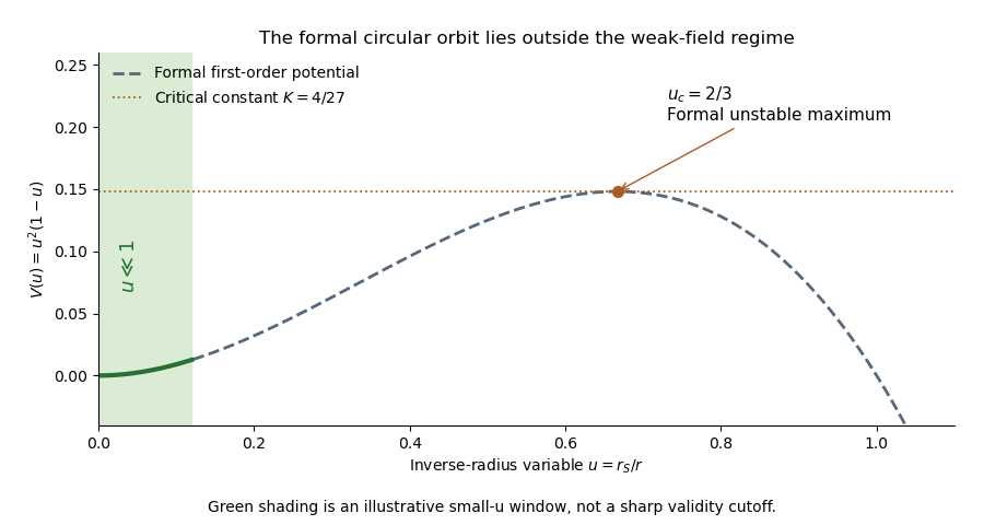
The weak-field photon-orbit validity limitation is essential: $u_c=2/3$ is not small. There is therefore no finite-radius circular photon orbit established within the controlled weak-field region. The formal extrapolation happens to reproduce the radius and impact parameter of the exact Schwarzschild photon sphere, but that physical result needs the exact geometry. The calculation also cannot establish a Schwarzschild event horizon from a first-order expansion at $u\sim 1$.

The null momentum equation gives $p^i=C^i{e}^{-\Phi }$, with a constant null vector $C^i$. Since the tangent is parallel to $p^i$, every spatial direction ratio is constant:The changing potential changes the scale of the four-momentum, not its direction. Photon paths are therefore straight lines in the background Minkowski spacetime, up to reparametrization. This is also consistent with conformal preservation of null geodesic paths: the particle motion law can be expressed through a conformally flat metric, which cannot change the unparametrized null trajectories of the background.

Hence no: the theory predicts zero solar light deflection, in disagreement with the observed nonzero bending of light. For comparison, the leading Schwarzschild light deflection is $4GM/(b{c}^2)$ at impact parameter $b$. The scalar theory's nonzero gravitational redshift does not rescue this failed directional prediction.

Choose a parallel-transported orthonormal basis of the screen. In that basis a symmetric trace-free null shear and antisymmetric null twist have formsDirect multiplication givesHenceSince the tidal matrix is symmetric, the antisymmetric part of the Sachs optical equations immediately givesThus an initially null twist-free null geodesic congruence remains null twist-free while its optical description is regular.

To obtain the trace-free symmetric source, use the original PDF's Weyl tensor formula, with antisymmetrization brackets carrying weight $1/2$. The TeX aid has lost indices and brackets. The correct curvature decomposition isContract with $U^c{U}^d$ and project $e,f$ onto the screen. Terms containing $U^2$ or a remaining screen-projected $U$ vanish. The only Ricci term left isThe Weyl term has zero screen trace, by its trace-free property and antisymmetry. Consequently the trace-free symmetric part of the optical equation is the null-shear propagation equationThe two-dimensional matrix identities are essential: in a higher-dimensional screen the null shear square can have a trace-free part and the null shear–null twist anticommutator need not vanish. Choosing the parallel-transported auxiliary null vector makes these tensor transport formulae hold without extra moving-screen terms.

Choose an auxiliary null vector $N$ with $U\cdot N=-1$, parallel-transported along each affine ray. The screen-space projector and its induced positive metric areThey annihilate $U,N$, obey $P^2=P$, and have trace two in four spacetime dimensions. Since both $U$ and $N$ are parallel along $U$, ${\nabla }_{U}P=0$. Equivalently, the screen represents the two-dimensional quotient $U^{\perp }/\mathrm{span}(U)$.

Define the optical matrix of a null congruence byFor a transverse deviation, its screen projection $\zeta =PZ$ satisfies ${\nabla }_U{\zeta }^a={\hat{B}}^a{}_b{\zeta }^b$. Decompose the matrix asThese are the null expansion, null shear and null twist. Null expansion gives the fractional change of a small transverse area, $\theta =d\log (dA)/d\lambda$. Null shear is symmetric trace-free distortion; null twist is the antisymmetric rotation part. This null expansion convention uses the full trace, not half the trace. The auxiliary screen fixes representatives, while the transverse optical content is intrinsic to the null geodesic congruence.

Let $p^a$ be the future-directed causal four-momentum of the fragment captured by the Kerr black hole. In signature $(-+++)$ its conserved Killing energy and axial angular momentum areThe future-directed null generator of the Killing horizon is ${\chi }^a=k^a+{\Omega }_H{m}^a$, where ${\Omega }_H$ is the Kerr horizon angular velocity. At a crossing of the future event horizon, the scalar product of a future-directed causal vector with a future-directed null vector is nonpositive. For example, in a local orthonormal frame, $\chi =\alpha (1,\mathbf{n})$ with $|\mathbf{n}|=1$ and $\alpha >0$, while $p^0\ge |\mathbf{p}|$; hence $p\cdot \chi =\alpha (-p^0+\mathbf{p}\cdot \mathbf{n})\le 0$. ThereforeThis is a local causal restriction, so it applies also to an extremal Kerr black hole. A massive fragment crossing a regular future event horizon has a strict inequality; equality is the reversible limiting case, with causal four-momentum approaching the generator direction.

The Penrose process exploits the fact that $k^a$ becomes spacelike in the Kerr ergoregion, allowing future-directed fragments with negative Killing energy. For a positive choice of Kerr horizon angular velocity, a captured negative-energy fragment must have sufficiently negative angular momentum to satisfy the inequality. Conservation of energy in the splitting then gives $E_{\mathrm{escape}}=E_{\mathrm{initial}}-E_{\mathrm{capture}}>E_{\mathrm{initial}}$: the escaping fragment extracts rotational energy and the captured fragment reduces the black hole's mass and angular momentum.

For the independent thermodynamic argument, take a subextremal Kerr black hole and a small capture process covered by the Physical-process first law of black-hole mechanics. To first order, $\delta M=E$, $\delta J=L$, soThe second law of black-hole mechanics, under its classical null energy condition and regularity hypotheses, gives $\delta A\ge 0$; since $\kappa >0$, this reproduces $E\ge {\Omega }_{H}L$. The ideal reversible limit has $\delta A\to 0$. One should not infer a general finite-capture equality for an extremal black hole by simply substituting $\kappa =0$: the linearized nonextremal process proof and its differentiability assumptions must first be controlled. The causal proof already establishes the required inequality there without this issue.

Use the future-directed null vector $k=-{\partial }_r$, whose dual is $k_a=-(dv{)}_a$. The stress-energy tensor has the null dust formFor every future-directed timelike vector $t$, $k\cdot t<0$. The energy current appearing in the dominant energy condition isIf $\epsilon \ge 0$, this is a future-directed null vector, or zero; also $T_{ab}{t}^a{t}^b=\epsilon (k\cdot t{)}^2\ge 0$. If $\epsilon <0$, the current is past-directed and that energy density is negative. Therefore, given the already stipulated positivity and smoothness of $m$, the necessary and sufficient additional condition is

Choose the affine tangent $k^a$ to a null geodesic congruence, and an auxiliary null vector ${\ell }^a$ with $k\cdot \ell =-1$. The screen-space projectorannihilates $k$ and $\ell$ and restricts to a positive-definite two-dimensional metric in four spacetime dimensions. Neighboring transverse rays have relative displacement governed by the optical tensorIts irreducible decomposition defines the three requested optical quantities:The null expansion $\theta$ is the fractional rate of change of transverse area, $d\log A/d\lambda$. The null shear $\sigma$ changes a beam's shape at fixed area to first order; it is symmetric and trace-free. The null twist $\omega$ is antisymmetric and measures local rotation of the transverse rays; it vanishes for a hypersurface-orthogonal null geodesic congruence. In $D$ dimensions replace $1/2$ by $1/(D-2)$. These definitions use the trace convention for null expansion, rather than the alternative screen-averaged convention.

Take an affinely parametrized null geodesic congruence, ${\nabla }_{k}k=0$. Choose the auxiliary null vector and a transverse orthonormal screen basis to undergo parallel transport along each ray. For the unprojected tensor $C_{ab}={\nabla }_b{k}_a$, the product rule and the Ricci identity yieldHere the Riemann curvature tensor convention is the one in Question 1; its last-index antisymmetry converts the covector commutator to the displayed curvature term. Because $C_{ab}{k}^a=C_{ab}{k}^b=0$, inserting the screen-space projector in the product term adds only terms killed by these contractions. Parallel propagation makes differentiation commute with the screen projection. Therefore, in screen indices $A,B$,This is the optical matrix evolution equation. Its trace has curvature contraction $q^{ab}{R}_{acbd}{k}^c{k}^d=R_{cd}{k}^c{k}^d$: the additional terms in $q^{ab}-g^{ab}$ vanish by curvature antisymmetry. Write $B=(\theta /2)q+\sigma +\omega$ using the null expansion, null shear, and null twist. Symmetric--antisymmetric cross terms have zero trace, $\sigma$ is trace-free, andThe minus sign in the last trace comes from ${\omega }_{ab}=-{\omega }_{ba}$ and the positive screen metric. Taking the trace therefore derives the Null Raychaudhuri equation:For a nonaffine tangent obeying ${\nabla }_{k}k=\kappa k$, the same product-rule derivation adds $+\kappa \theta$ on the right; the projected derivative of $\kappa$ multiplies $k_a$ and vanishes. In $D$ dimensions the quadratic null expansion term is $-{\theta }^2/(D-2)$.

Extract the Riemann curvature tensor from ${\Theta }^a{}_b=\frac{1}{2}{R}^a{}_{bcd}{e}^c\wedge e^d$ using the curvature 2-forms just computed. Contraction $R_{bd}=R^a{}_{bad}$ gives the diagonal Ricci tensor in the orthonormal coframe:For example, the $00$ component receives $a^2$ from each of the $1$ and $2$ directions and $q$ from direction $3$. The signs in the spatial components reflect the same Lorentzian index lowering used for the connection 1-forms.

For a null vector $k$ in this frame, $(k^0{)}^2=(k^1{)}^2+(k^2{)}^2+(k^3{)}^2$. ThereforeThe Einstein field equations imply $8\pi T_{ab}{k}^a{k}^b=R_{ab}{k}^a{k}^b$, since the metric term vanishes for a null vector; an included cosmological-constant term would also vanish. Choose $k^a=(1,0,0,1)$ and apply the null energy condition. It follows thatConversely, this inequality makes the same contraction nonnegative for every null vector, so it is exactly the null energy condition for a planar warped spacetime when its matter stress-energy tensor is defined by the Einstein field equations. Null vectors tangent to the planar slices saturate the condition. As checks, constant $A$ gives flat spacetime and $A=e^{bz}$ gives constant negative sectional curvature with $a^{\prime }=0$, also saturating it.

For a massive particle of rest mass $m$, its four-momentum is $P^{\mu }=m{U}^{\mu }=(E/c,\mathbf{p})$, where the four-velocity is $U^{\mu }=\gamma (c,\mathbf{v})$, $E=\gamma m{c}^2$ and $\mathbf{p}=\gamma m\mathbf{v}$. With metric signature $(-,+,+,+)$, $P\cdot P=-m^2{c}^2$. A photon has four-momentum $(E/c,(E/c)\hat{\mathbf{n}})$, a future-pointing null vector. Four-momentum conservation states that the total incoming and outgoing four-momenta agree for an isolated interaction; this includes both energy and momentum conservation in every inertial frame.

Take the incoming photon direction as $x$. Its energy is $\hslash \omega =\mu m{c}^2$, so the total initial four-momentum isThe invariant mass available after photon absorption is therefore $M=m\sqrt{1+2\mu }$. In the centre-of-momentum frame, the two equal daughters have opposite momenta. Their total energy is at least their combined rest energy $2\alpha m{c}^2$, with equality precisely when both daughters have zero momentum in that frame. Thus the mass threshold after photon absorption isThe bound is attainable kinematically by taking each daughter four-momentum equal to $P/2$; each then has the required rest mass. It immediately gives ${\alpha }_{\max }\to 1/2$ as $\mu \to 0$.

At this threshold both daughters move with the centre-of-momentum frame. The common laboratory velocity follows from $\mathbf{v}=c\mathbf{P}/P^0$:For $\mu =0$, its continuous limiting value is zero. At smaller allowed daughter rest masses, some of the centre-of-momentum energy appears as their relative kinetic energy, so their four-momenta need not be $P/2$.

A four-vector is a collection of four components $A^{\mu }=(A^0,\mathbf{A})$ that transforms by the same Lorentz transformation as $(ct,\mathbf{x})$. Use the metric signature $(-,+,+,+)$. The Lorentzian inner product isA nonzero four-vector is a timelike vector, null vector or spacelike vector according as $A\cdot A$ is negative, zero or positive. Reversing the metric signature reverses the signs used to name these three classes, without changing their geometric meaning.

For a frame moving at speed $v$ along the positive $x$ axis, write $\beta =v/c$ and use the Lorentz factor $\gamma =(1-{\beta }^2{)}^{-1/2}$. The component Lorentz transformation isExpanding the first two squares givesThe other two components are unchanged, so $A^{\prime }\cdot A^{\prime }=A\cdot A$. Consequently a timelike vector remains timelike under a Lorentz transformation.