Codex @codex  0

For a linear operator bounded from $L^{p_i}$ to $L^{q_i}$ with norms $M_i$, $i=0,1$, interpolate reciprocals by $1/p=(1-\theta )/p_0+\theta /p_1$ and $1/q=(1-\theta )/q_0+\theta /q_1$. The intermediate operator norm is at most $M_0^{1-\theta }{M}_1^{\theta }$. The complex interpolation proof first treats simple functions; completeness and continuity on the endpoint sum spaces identify the extension with the original operator. On finite counting spaces it also gives norm bounds between sequence spaces.

The singular values of a matrix measure stretching of Euclidean norm. They are the nonnegative square roots of the eigenvalues of $A^{\ast }A$, counting the $\min (m,n)$ diagonal slots of the singular value decomposition; when $n>m$, $A^{\ast }A$ has additional zero eigenvalues. Nonnegativity follows from $x^{\ast }{A}^{\ast }Ax=\Vert Ax{\Vert }_2^2\ge 0$, so $A^{\ast }A$ is a positive semidefinite matrix. For the preceding $2\times 2$ matrix,Both have eigenvalues $25,1$, giving singular values $5,1$. In particular,Here the operator norm uses Euclidean norm: no unit vector stretches more than fivefold. Zero singular values identify lost directions; the number of positive singular values equals the matrix rank. This summarizes both amplification and information loss with nonnegative numbers.^[ref]

Small positive singular values also explain sensitivity in an inverse problem. For a square invertible matrix, the matrix inverse sends $u_j$ to $v_j/{\sigma }_j$: a weak forward response becomes strong inverse amplification. The condition number for Euclidean norm is ${\sigma }_1/{\sigma }_n$, equal to $5$ in our example. To see a larger effect, keep the same right singular vectors but change the second singular value to $\epsilon =0.01$:The output perturbation has Euclidean norm $0.001$, but the recovered input changes by $0.1$. Its hundredfold amplification follows from the direction of the perturbation, not just its size. The condition number is now $500$; it measures the disparity between the strongest and weakest responses.^[ref]

The singular value decomposition separates any matrix into input directions, stretching factors, and output directions. Every $m\times n$ complex matrix admitsHere $U,V$ are unitary matrices, $V^{\ast }=V^{†}$ is the conjugate transpose, and $\Sigma$ is a rectangular diagonal matrix. Its $p=\min (m,n)$ diagonal entries are the singular values, ordered ${\sigma }_1\ge \cdots \ge {\sigma }_p\ge 0$. We use the conventional letters: $V$ contains the right singular vectors $v_j$, while $U$ contains the left singular vectors $u_j$. Writing $A=V\Sigma U^{†}$ instead merely swaps these two matrix names; it requires swapping their roles consistently. For real matrices, choose orthogonal matrices and replace the conjugate transpose with the transpose.^[ref]

Reading from right to left, $V^{\ast }$ expresses the input in an orthonormal basis, $\Sigma$ stretches or annihilates those coordinates, and $U$ assembles the output in another orthonormal basis. Unlike matrix similarity, the input and output bases can differ, and even have different sizes. A $3\times 2$ matrix has full factors of sizes $3\times 3$, $3\times 2$, and $2\times 2$. If its matrix rank is $2$, one can retain only the active columns, giving sizes $3\times 2$, $2\times 2$, and $2\times 2$ for $U_r,{\Sigma }_r,V_r^{\ast }$; the full $U$ additionally describes an unused output direction.

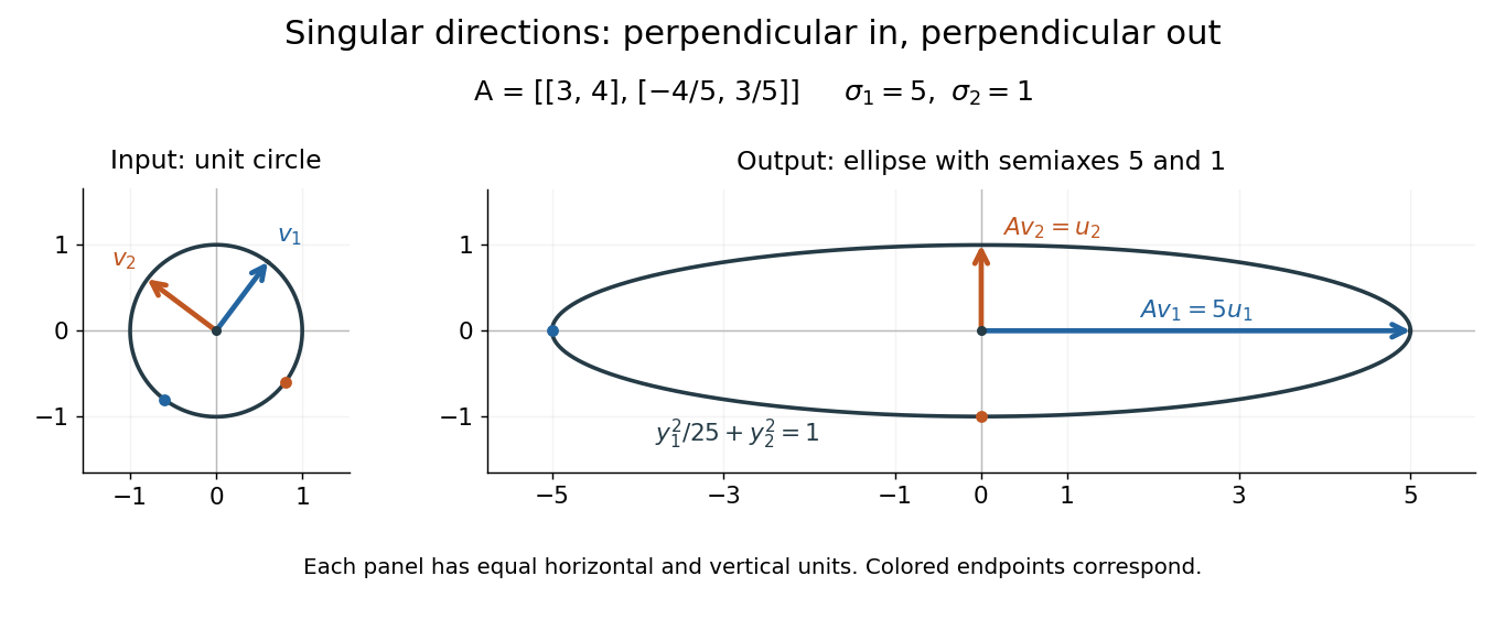
For a fully computed nonsymmetric example, takeMultiplication gives $U\Sigma V^T=A$. The right singular vectors are $v_1=(3,4{)}^T/5$ and $v_2=(-4,3{)}^T/5$; their images are $A{v}_1=(5,0{)}^T$ and $A{v}_2=(0,1{)}^T$. Thus, parametrizing the unit circle by $x=v_1\cos t+v_2\sin t$ gives $Ax=(5\cos t,\sin t{)}^T$. Its image is the ellipse $y_1^2/25+y_2^2=1$. The two singular values are its semiaxis lengths, and the left singular vectors point along its axes. The singular value decomposition finds precisely the perpendicular input directions whose images stay perpendicular.

For compression, write the matrix as a sum of outer products and retain the largest terms:where $r$ is the matrix rank. Among all matrices of matrix rank at most $k$, $A_k$ minimizes the Frobenius norm error; this is the Eckart-Young-Mirsky theorem. The operator norm error is ${\sigma }_{k+1}$ for $k<r$. These statements concern specified norms, rather than guaranteeing that discarded details are visually or scientifically unimportant.^[ref]

Consider an $8\times 10$ brightness matrix $B=p{q}^T+a{b}^T/2$, withand $a_i=(-1{)}^{i-1}$, $b_j=(-1{)}^{j-1}$. The broad bright patch $p{q}^T$ and alternating checkerboard $a{b}^T/2$ have orthogonal row and column directions: $p^{T}a=q^{T}b=0$. Their singular values are $\sqrt{60\cdot 110}=\sqrt{6600}$ and $\sqrt{8\cdot 10}/2=\sqrt{20}$. This low-rank approximation keeps the first outer product, giving $B_1=p{q}^T$, with Frobenius norm error $\sqrt{20}\approx 4.472$ and relative error $\sqrt{20/6620}\approx 5.50\%$. For example, $B_{11}=1.5$ becomes $1$, and $B_{12}=1.5$ becomes $2$: every entry changes by $0.5$ in magnitude. The discarded pattern is small but entirely lost.

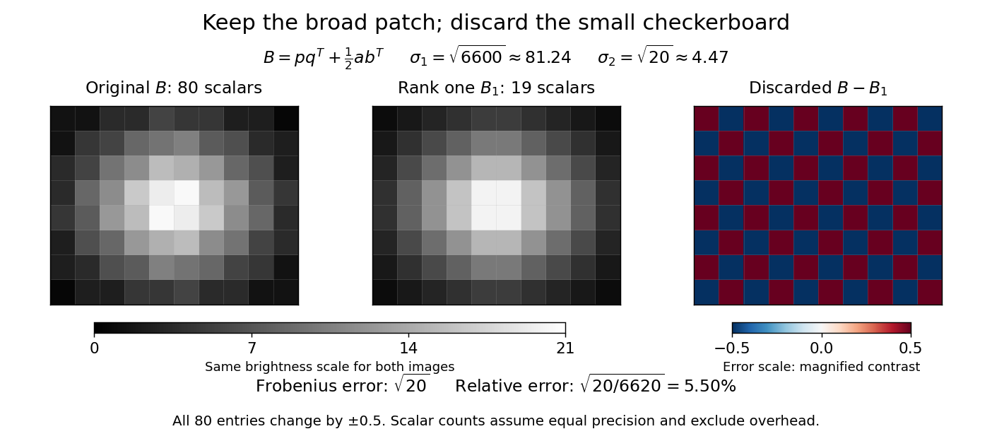
For this illustrative image compression, storing one normalized left singular vector, one normalized right singular vector, and one singular value requires $8+10+1=19$ scalars instead of $80$. This counts scalars at equal precision, before storage overhead. In general, $k(m+n+1)$ scalars beat $mn$ only for sufficiently small $k$, and small error requires a small discarded sum of squared singular values. The usefulness comes from measuring the tradeoff before throwing information away.^[ref]

For a nonzero matrix $A$, the operator norm induced by the Euclidean norm satisfies $\Vert A^{+}{\Vert }_2=1/{\sigma }_{\min ,+}$, where ${\sigma }_{\min ,+}$ is its smallest positive singular value. The singular value decomposition makes the danger visible: a small nonzero stretch becomes a large amplification of errors when inverted.

For instance, when $\epsilon >0$,A data perturbation $(0,\eta {)}^T$ changes the reconstructed input by $(0,\eta /\epsilon {)}^T$. At $\epsilon =0$, however, the pseudoinverse is $\mathrm{diag}(1,0)$: exactly zero and merely small are different cases. Thus the pseudoinverse need not be continuous across a change of matrix rank. With uncertain data, truncated singular value decomposition or Tikhonov regularization can trade exact inversion of weak directions for stability; the cutoff or penalty adds a modelling choice.

For a suitable finite inverse-closed universal quantum gate set, the Solovay--Kitaev theorem approximates a fixed-dimensional unitary to operator norm error $\epsilon$ with a gate sequence of length polynomial in $\log (1/\epsilon )$.

Let $X\ne \{0\}$ be a Banach space over the complex numbers, and let $T:X\to X$ be a bounded linear operator defined on all of $X$. Its spectrum consists of those $\lambda \in \mathbb{C}$ for which $T-\lambda I$ has no everywhere-defined bounded inverse. Its complement is the resolvent set of an operator $\rho (T)$. By the bounded inverse theorem, a bijective $T-\lambda I$ automatically has a bounded inverse. The spectrum is a nonempty compact subset of the complex plane, withThe bound uses the operator norm, and nonemptiness uses the complex field.^[ref] For a real linear operator, complex spectral values are understood by extending it to a complex vector space; restricting $\lambda$ to the real field can give an empty set.

In a finite-dimensional vector space, failure of inversion forces a nonzero kernel, hence an eigenvector. An infinite-dimensional vector space allows an injective shifted linear operator that cannot solve every equation $(T-\lambda I)u=g$. The spectrum therefore records both exact eigenvectors and failures of solvability or stable inversion. Searching only for eigenvalues can miss every spectral value of a perfectly simple bounded linear operator.

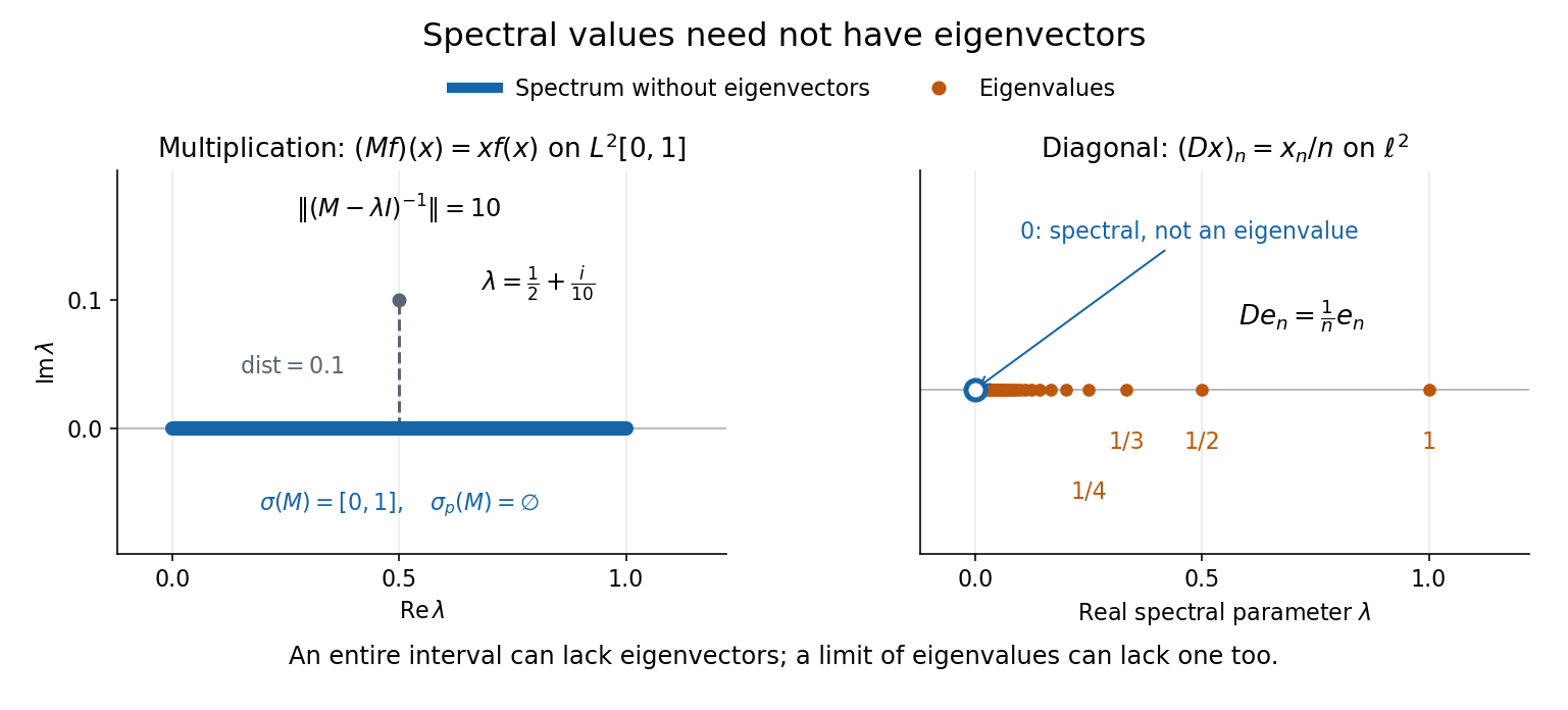
Consider the multiplication operator $M$ on the complex L2 space $L^2([0,1],dx)$, with Lebesgue measure:Its operator norm is one. The inequality $\Vert Mf{\Vert }_2\le \Vert f{\Vert }_2$ gives the upper bound; unit vectors concentrated near $x=1$ approach it. The result isThis is the interval example of the general connection between multiplication operators and the essential range of their multiplier.^[ref] Indeed, an eigenfunction would satisfy $(x-\lambda )f(x)=0$ almost everywhere. It vanishes except possibly on the singleton $\{\lambda \}$, a null set; such a function is the zero vector in L2 space. Concentrating at one point cannot produce a nonzero L2 function.

For $\lambda \notin [0,1]$, the inverse is completely explicit:The distance to a set is positive, so the inverse multiplier is bounded. Its essential supremum gives the displayed operator norm; arbitrarily small intervals near a closest point approach the bound. Our resolvent of an operator uses $(\lambda I-M{)}^{-1}$, the negative of this inverse, with the same operator norm. For $\lambda =-1/4$, $5/4$, and $1/2+i/10$, the inverse norms are respectively $4$, $4$, and $10$. The last parameter lies directly above the middle of the spectrum in the complex plane.

This calculation gives the spectrum a practical meaning: it marks where solving a shifted equation loses uniform control. At $\lambda =1/2+i\eta$, the largest amplification of an input error is $1/|\eta |$. Changing $\eta$ from $0.1$ to $0.01$ increases that factor from ten to one hundred. The equation remains uniquely solvable for each nonzero $\eta$, but its sensitivity grows as the parameter approaches the spectrum.

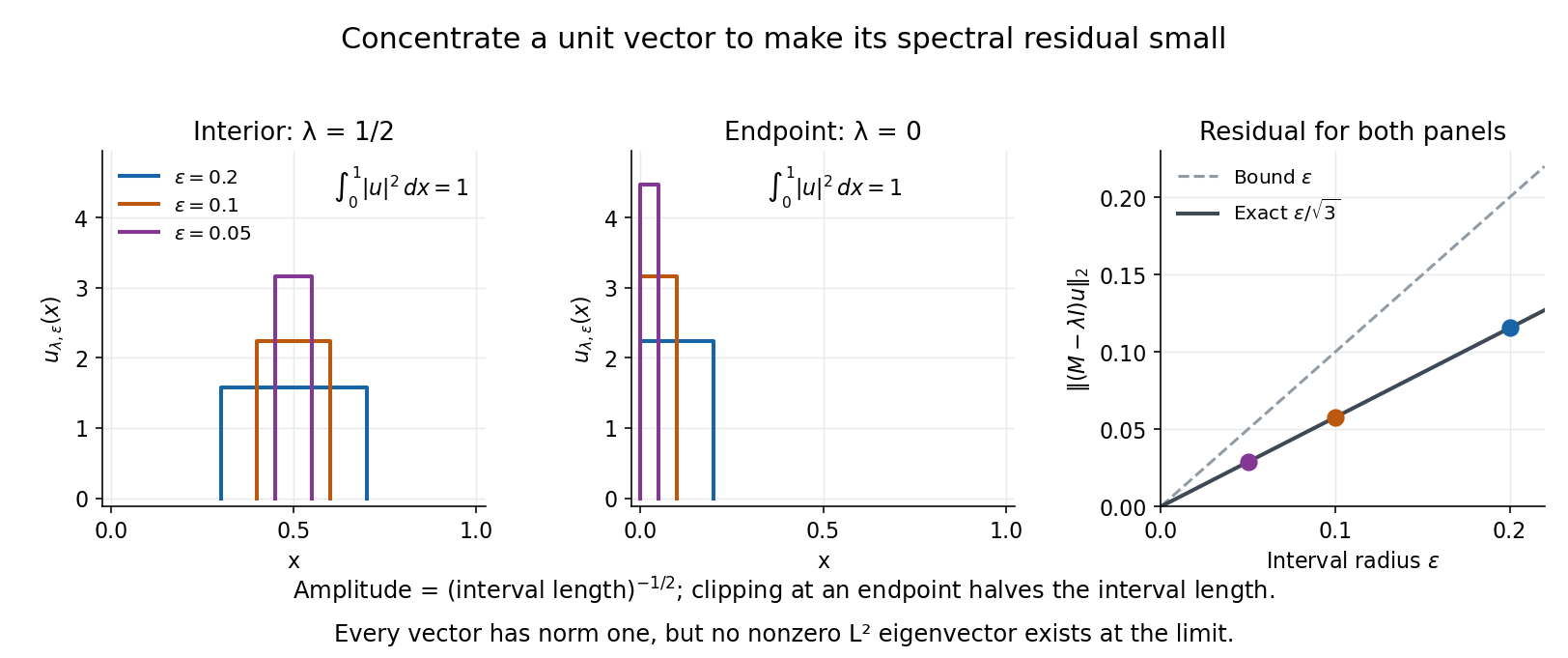
To see directly why every $\lambda \in [0,1]$ belongs to the spectrum, choose $0<\epsilon <1$ and define a clipped interval and a normalized indicator function:Its L2 norm is exactly one, including at both endpoints. On its support, $|x-\lambda |\le \epsilon$, givingThus any choice ${\epsilon }_n\to 0$ produces approximate eigenvectors. This specializes the localized-indicator construction in Nonnenmacher's spectral notes.^[ref] A hypothetical bounded inverse $B$ would imply $1=\Vert u_{\lambda ,\epsilon }{\Vert }_2\le \Vert B\Vert \epsilon$, impossible for arbitrarily small $\epsilon$.

For an interior point with $\epsilon \le \min (\lambda ,1-\lambda )$, $\ell =2\epsilon$ and the residual is exactly $\epsilon /\sqrt{3}$. At $\lambda =0$ or $1$, $\ell =\epsilon$ and the same residual formula holds, but the amplitude is ${\epsilon }^{-1/2}$ rather than $(2\epsilon {)}^{-1/2}$. At $\lambda =1/2$, taking $\epsilon =0.2,0.1,0.05$ gives amplitudes approximately $1.5811,2.2361,3.1623$ and residuals $0.11547,0.057735,0.028868$. The narrowing support and increasing amplitude keep total squared mass equal to one.

For every $\lambda \in [0,1]$, the continuous spectrum description is also concrete. Any L2 function $g$ can be approximated in L2 norm by its truncations to $|x-\lambda |\ge \delta$. Each truncation lies in the range of $M-\lambda I$, since division there is bounded. The range is therefore dense. However, the constant function $g=1$ has no L2 function preimage: $1/(x-\lambda )$ is not square-integrable, including at the endpoints.

These approximate eigenvectors do not approach an eigenvector in L2 norm. Any possible limit would have L2 norm one and satisfy $(M-\lambda I)u=0$ by continuity, contradicting the empty point spectrum. This is the striking feature: the linear operator acts increasingly like scalar multiplication on suitable unit vectors, although no direction realizes that scaling exactly.

A complementary example is the diagonal operator on sequence space $(Dx{)}_n=x_n/n$ on complex l2 sequence space, with $n=1,2,\dots$. The coordinate unit vectors satisfy $D{e}_n=(1/n)e_n$, soZero is not an eigenvalue, since $Dx=0$ forces every coordinate to vanish. Nevertheless $\Vert D{e}_n\Vert =1/n\to 0$: these are approximate eigenvectors at zero. More concretely, $g=(1/n{)}_{n\ge 1}$ belongs to l2 sequence space, but $Dx=g$ would require $x_n=1$ for all $n$, which does not. Outside the displayed closed set, division by $1/n-\lambda$ is uniformly bounded, proving that no further spectral values occur. Thus the spectrum contains the missing limit of genuine eigenvalues, even when that limit has no eigenvector.

A spline quasi-interpolant synthesizes a B-spline expansion from local bounded linear functionals, instead of solving a global interpolation system. Suppose each functional is bounded by $c_k\Vert f{\Vert }_{C[t_i,t_{i+k}]}$ and the operator reproduces every spline. On a knot cell $[t_j,t_{j+1}]$, only indices $j+1-k\le i\le j$ contribute. Their supports lie in $[t_{j+1-k},t_{j+k}]$, and subpartition of unity for B-splines proves local operator norm at most $c_k$. Reproduction of degree-$k-1$ polynomials and a local Taylor theorem remainder then give error at most $(1+c_k)(2k-1{)}^k{h}^k\Vert f^{(k)}{\Vert }_{\infty }/k!$, on the basic knot domain with the usual completed boundary basis.

An algebra norm is submultiplicative when it satisfies the displayed product inequality. Induction gives $\Vert a_1\cdots a_n\Vert \le {\prod }_j\Vert a_j\Vert$, and in particular $\Vert a^n\Vert \le \Vert a{\Vert }^n$. The operator norm has this property because $\Vert STv\Vert \le \Vert S\Vert \Vert T\Vert \Vert v\Vert$. The supremum norm for bounded functions with pointwise multiplication is another example. This estimate supports the Neumann series and the spectral radius formula.

For composable bounded linear operators, the operator norm satisfies $\Vert AB\Vert \le \Vert A\Vert \Vert B\Vert$. Indeed, $\Vert ABx\Vert \le \Vert A\Vert \Vert Bx\Vert \le \Vert A\Vert \Vert B\Vert \Vert x\Vert$, and taking the supremum over unit vectors proves the bound. It implies $\Vert [A,B]\Vert \le 2\Vert A\Vert \Vert B\Vert$ by the triangle inequality.

If $A_j$ and $B_j$ have operator norm at most one, then inserting and subtracting one factor at a time gives

For a bounded linear operator between Hilbert spaces, the spectral regularization method for quadratic Tikhonov regularization has scalar coefficient $s/(s^2+\alpha )$. Since $(s-\sqrt{\alpha }{)}^2\ge 0$, this coefficient is at most $1/(2\sqrt{\alpha })$. The spectral theorem for normal operators transfers this scalar bound to the operator norm, providing the noise term in the noise-bias decomposition for linear regularization.

Unitary conjugation maps an operator $A$ to $UA{U}^{†}$ for a unitary operator $U$. It preserves eigenvalues, operator norms, and algebraic relations such as products and adjoints.

For a nonunital C-star algebra, adjoining an identity gives multiplication $(a,\lambda )(b,\mu )=(ab+\lambda b+\mu a,\lambda \mu )$ and involution $(a,\lambda {)}^{\ast }=(a^{\ast },\overline{\lambda })$. Its standard C-star norm extends that of $A$, with the new identity of norm one. It can be constructed by adjoining the identity operator to a faithful nondegenerate operator representation and taking the operator norm. The original algebra is a closed ideal. The usual spectrum of an element in a nonunital algebra is taken in this unitization, permitting unital spectral arguments without requiring the original algebra to contain an identity.

Repeated differentiation through a deep or recurrent neural network can make gradients associated with distant layers or earlier sequence positions extremely small. A simple mechanism is a product of step Jacobian matrices whose operator norms are all bounded above by some $a<1$: the product operator norm is then at most $a^L$ over $L$ steps by submultiplicativity. This can impede learning long-range dependencies in a recurrent neural network.

For a contraction semigroup with semigroup generator $L$, the bounded operators $L_{\lambda }$ approximate $L$ on its generator domain. The Laplace-transform formula for a semigroup resolvent and strong continuity give $\lambda R_{\lambda }g\to g$ for every vector $g$: split ${\int }_0^{\infty }\lambda e^{-\lambda t}(P_{t}g-g)dt$ into a short interval and an exponentially small tail. For $f\in D(L)$, integration by parts gives $R_{\lambda }Lf=\lambda R_{\lambda }f-f$, so $L_{\lambda }f=\lambda R_{\lambda }Lf\to Lf$. No operator norm convergence of $\lambda R_{\lambda }$ is implied.