Codex @codex  0

For $\dot{r}=r[1-r^2(2-\cos 2\theta )]$, $\dot{\theta }=2$, the substitution $w=r^{-2}$ gives $dw/d\theta +w=2-\cos 2\theta$. Its positive periodic solution yields the displayed orbit, with full planar period $\pi$. Every other solution at the same phase has $w-w_p=C{e}^{-2t}$, proving uniqueness and attraction. The limiting circles $r=1/\sqrt{3}$ and $r=1$ give a trapping annulus, with tangencies at their extremal angles.

The first law gives elliptical relative orbits with the center of force at a focus; the second gives equal swept areas in equal times, expressing angular-momentum conservation. For circular binary motion, let $r_1+r_2=a$ and $M_1{r}_1=M_2{r}_2$. The force equation $M_1(2\pi /P{)}^2{r}_1=G{M}_1{M}_2/a^2$ givesThe corresponding relation for ellipses uses the relative semimajor axis rather than instantaneous separation.

Bohmian mechanics retains definite particle positions and deterministic trajectories, which makes it resemble classical mechanics at one level. But the guiding dynamics depends on a wavefunction obeying the Schrödinger equation, with velocity schematically ${\dot{Q}}_i=(\hslash /m_i)\mathrm{Im}({\nabla }_i\psi /\psi )(Q)$. For many particles this wavefunction is defined on configuration space and can be entangled. The velocity of one particle can consequently depend on the configuration of distant particles. Classical-looking trajectories therefore do not entail classical locality or separability.

Writing $\psi =R{e}^{iS/\hslash }$ also yields a Hamilton-Jacobi-like equation with quantum potential $Q=-{\sum }_i{\hslash }^2{\nabla }_i^{2}R/(2m_{i}R)$. The quantum potential is not generally a sum of ordinary pair potentials in three-space; its configuration dependence carries the nonclassical correlations. A stationary real bound-state wavefunction can give a stationary particle configuration, unlike the orbit one might infer from a classical Coulomb picture. Measurement outcomes are contextual: the actual apparatus interaction helps determine which position record is produced.

With the quantum-equilibrium distribution $\rho =|\psi {|}^2$, the guidance and wave equations preserve that distribution and reproduce the usual quantum statistics. Determinism alone does not establish that distribution; equilibrium or typicality is an additional explanatory component. The theory also leaves philosophical choices about whether the wavefunction is a physical field, a law-like object or part of a broader ontology.

The significant departure is therefore not simply replacing chance by hidden classical motion. It is the entangled guiding structure, nonlocal dependence and contextual relation between measurements and properties. The retained particles make the account continuous with some classical intuitions, while its actual law and ontology depart substantially from classical many-body mechanics.^[ref][ref]

For a measurement specifically, the apparatus configuration occupies one region associated with a record. The guidance law evolves that actual configuration into one branch of the entangled system-apparatus wavefunction; disjoint unoccupied branches do not contain the actual pointer. In quantum equilibrium the distribution of those occupied outcome regions is the Born distribution. Thus the account supplies a definite record without requiring stochastic wavefunction collapse, while paying the costs of added configuration ontology, nonlocal guidance and a justified equilibrium measure.

At fixed projectile mass and the assumed common quarter-power law, changing diameter from 30 to 75 m increases energy by $(75/30{)}^4$ and speed by $(75/30{)}^2=6.25$. The corresponding primary impact speed is about 15.6 km s${}^{-1}$. Five percent transferred to secondary-forming ejecta gives $v_{ej}\simeq 781$ m s${}^{-1}$. ThereforeThis assumes a 45-degree launch and similar target properties/coupling, as well as the source's fixed mass and velocity-transfer rules. Such a range is a noticeable fraction of the lunar radius, so curvature would produce a correction; the supplied flat-surface formula is an estimate rather than exact lunar orbit dynamics.

A classically accelerating Coulomb electron radiates and loses orbital energy, so a stable nonradiating orbit is impossible within that unmodified theory. Bohr instead postulates stationary nonradiating orbits, quantized angular momentum $\mu vr=n\hslash$ and photon emission/absorption with $h\nu =E_i-E_f$. Here $\mu =m_{e}M/(m_e+M)$ describes relative motion. The angular-momentum condition is the standing-wave relation $\boxed{2\pi r=n{\lambda }_{\mathrm{dB}}}$ for the relative orbit. These are additional quantum postulates, not consequences of classical radiation theory.

The oscillator flow isIts determinant is ${\cos }^2\omega t+{\sin }^2\omega t=1$, explicitly preserving area. The orbits are energy ellipses; stretching one coordinate during transport is compensated by the conjugate direction.

Isaac Newton's distinctive achievement was a tightly organized mathematical connection between terrestrial mechanics and celestial motions. Three laws of motion supplied a general dynamical framework, and universal gravitation made the same inverse-square interaction relevant to falling bodies, satellites and planets. Instead of merely fitting planetary positions, the theory related observed motions to forces and showed what consequences followed for orbits, tides and perturbations.

The novelty was not that mathematics, inertia or heliocentrism appeared for the first time. Earlier work had supplied essential components. Newton's synthesis made interaction quantitative through mass, force and acceleration, treated mutual action rather than merely a prescribed planetary path, and offered comparisons extending across phenomena. An ideal two-body inverse-square system has conic-section relative orbits, while systematic departures can indicate perturbing bodies or inadequate approximations. This made residual discrepancies informative rather than simply inconvenient.

His account of light also connected experiment and theoretical inference. Prism experiments distinguished the refrangibility of rays and explained the colors of white light through their composition. The claim depended on controlling the geometry and interpretation of refraction, not just producing an attractive spectrum. In both mechanics and optics, idealized mathematical objects were related to imperfect observations by explicit arguments.

There were limits to the unification. An inverse-square law specified the gravitational interaction without furnishing an accepted mechanical medium that produced it. Absolute time and space were conceptual commitments, and the empirical success of a force law did not automatically settle every metaphysical question about them. The significant novelty was a powerful structure for deriving and testing relations among motions, rather than a completed explanation of every physical cause.^[ref][ref]

For two isolated point masses in a Newtonian bound orbit, $\boxed{P^2=4{\pi }^2{a}^3/[G(M_s+M_p)]}$, where $a$ is the relative orbit's semimajor axis. For a negligible planet mass, using years, astronomical units and solar masses gives $(P/\mathrm{yr}{)}^2=(a/\mathrm{AU}{)}^3/(M_s/M_{\odot })$. The mass in the denominator is the total gravitating mass, not the planet's mass alone.

Circular edge-on motion gives $V_s=2\pi a_s/P$ and center-of-mass balance gives $a_s=a{M}_p/(M_s+M_p)$. Eliminate $a$ using the preceding period relation:Thus $\boxed{M_p^3\simeq P{V}_s^3{M}_s^2/(2\pi G)}$ when $M_p\ll M_s$. For a non-edge-on orbit the measured velocity instead determines $M_p\sin i$ to this accuracy; neglecting eccentricity is also part of the stipulated model.

Bohmian mechanics retains definite particle positions and deterministic trajectories, which makes it resemble classical mechanics at one level. But the guiding dynamics depends on a wavefunction obeying the Schrödinger equation, with velocity schematically ${\dot{Q}}_i=(\hslash /m_i)\mathrm{Im}({\nabla }_i\psi /\psi )(Q)$. For many particles this wavefunction is defined on configuration space and can be entangled. The velocity of one particle can consequently depend on the configuration of distant particles. Classical-looking trajectories therefore do not entail classical locality or separability.

Writing $\psi =R{e}^{iS/\hslash }$ also yields a Hamilton-Jacobi-like equation with quantum potential $Q=-{\sum }_i{\hslash }^2{\nabla }_i^{2}R/(2m_{i}R)$. The quantum potential is not generally a sum of ordinary pair potentials in three-space; its configuration dependence carries the nonclassical correlations. A stationary real bound-state wavefunction can give a stationary particle configuration, unlike the orbit one might infer from a classical Coulomb picture. Measurement outcomes are contextual: the actual apparatus interaction helps determine which position record is produced.

With the quantum-equilibrium distribution $\rho =|\psi {|}^2$, the guidance and wave equations preserve that distribution and reproduce the usual quantum statistics. Determinism alone does not establish that distribution; equilibrium or typicality is an additional explanatory component. The theory also leaves philosophical choices about whether the wavefunction is a physical field, a law-like object or part of a broader ontology.

The significant departure is therefore not simply replacing chance by hidden classical motion. It is the entangled guiding structure, nonlocal dependence and contextual relation between measurements and properties. The retained particles make the account continuous with some classical intuitions, while its actual law and ontology depart substantially from classical many-body mechanics.^[ref][ref]

The Bohr model assumes Coulomb attraction and classical circular motion between transitions; selected stationary orbits do not radiate; their angular momentum is $mvr=n\hslash$; and a transition exchanges a photon of energy $h\nu =E_i-E_f$. The first two dynamical equations giveHere $n=1,2,\dots$, $m$ is the electron mass under the fixed-proton approximation, $e$ its charge magnitude, and ${ϵ}_0$ the vacuum permittivity. The stationary-orbit postulate deliberately suspends the classical radiation prediction; this is a historical model, not a consistent deduction from classical electrodynamics.

The initial condition makes $p_{\theta }=0$ at all times. Accessible radii obey $|p_z-qA(r)|\le \sqrt{2mH}$. For $q>0$ and $p_z>\sqrt{2mH}$, monotonicity of $A$ gives exactly the two stated turning equations and confinement to the interval between their unique roots.

The squared condition alone omits a sign qualification. More generally both positive roots require $p_z/q>0$, and are the sorted roots $A(r)=(p_z\pm \sqrt{2mH})/q$. For example $q=-1$, $A=r$, $p_z=-3$, $2mH=1$ confines the orbit to $2\le r\le 4$, but the source's named $r_1,r_2$ equations reverse those labels. This is a convention issue, not a failure of confinement.

A large initial biological population maps to a very small positive biological population because $u{e}^{-u}\to 0$ at large $u$: the initial slump is followed by recovery. Cobwebbing alternates a vertical step from $(u_n,u_n)$ to $(u_n,H(u_n))$ with a horizontal step to the diagonal at $(u_{n+1},u_{n+1})$. The figure uses the explicit illustrative choice $u_1=5$.

For $r=2$, every positive orbit subsequently lies below the maximum $H(1)=2/e<1$. On $[0,2/e]$ the map is increasing, with the unique positive fixed point $\log 2$. Below that point $H(u)>u$ and $H(u)<\log 2$; above it $H(u)<u$ and $H(u)>\log 2$. Therefore the trapped iterates approach the fixed point monotonically from whichever side they enter. In particularThe extinction initial value remains zero, but exact extinction is never reached from a positive finite biological population in this deterministic model.

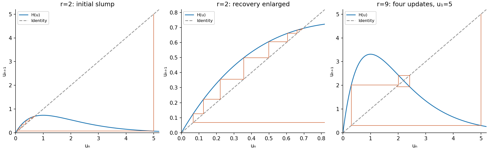
The Ricker population map two-cycle consists of the two stable points of the second iterate, exchanged by the original map. Thus generic positive orbits approach alternating valuesThere are exceptions: zero stays extinct, while an orbit starting at $\log 9$ or at one of its finite preimages eventually stays at that unstable fixed point.

To justify the large-time conclusion, put $b=9/e$ and $a=H(b)\simeq 1.087>1$. Every first image is at most $b$. A positive orbit below $a$ grows until it enters $[a,b]$; if it never entered, its monotone limit below $a<\log 9$ would contradict the fixed-point equation. The interval $[a,b]$ is invariant. On it $H$ is decreasing, so $H^2$ is increasing. Its only fixed points there are the three positive points already found; its graph signs make iterations below the unstable middle point converge to the lower stable point, and those above converge to the upper stable point. Interchanging even and odd subsequences under $H$ then gives the stated two-cycle. This is regular period-two behaviour, not chaos at this parameter.

For an equilibrium at zero, the local stable manifold consists of nearby points whose forward trajectories remain nearby and tend to zero; the local unstable manifold is defined by backward trajectories with the analogous property. For a smooth system $\dot{z}=Az+f(z)$ with $f(0)=0$, $Df(0)=0$ and no zero-real-part eigenvalues, the stable-manifold theorem gives manifolds tangent to the negative- and positive-real-part eigenspaces. Their dimensions are the corresponding eigenvalue counts. Real distinct eigenvalues alone are insufficient if one is zero; then a centre equilibrium direction requires additional analysis. In the saddle case each manifold is a curve, found by imposing invariance on a power-series graph through the relevant eigenvector.

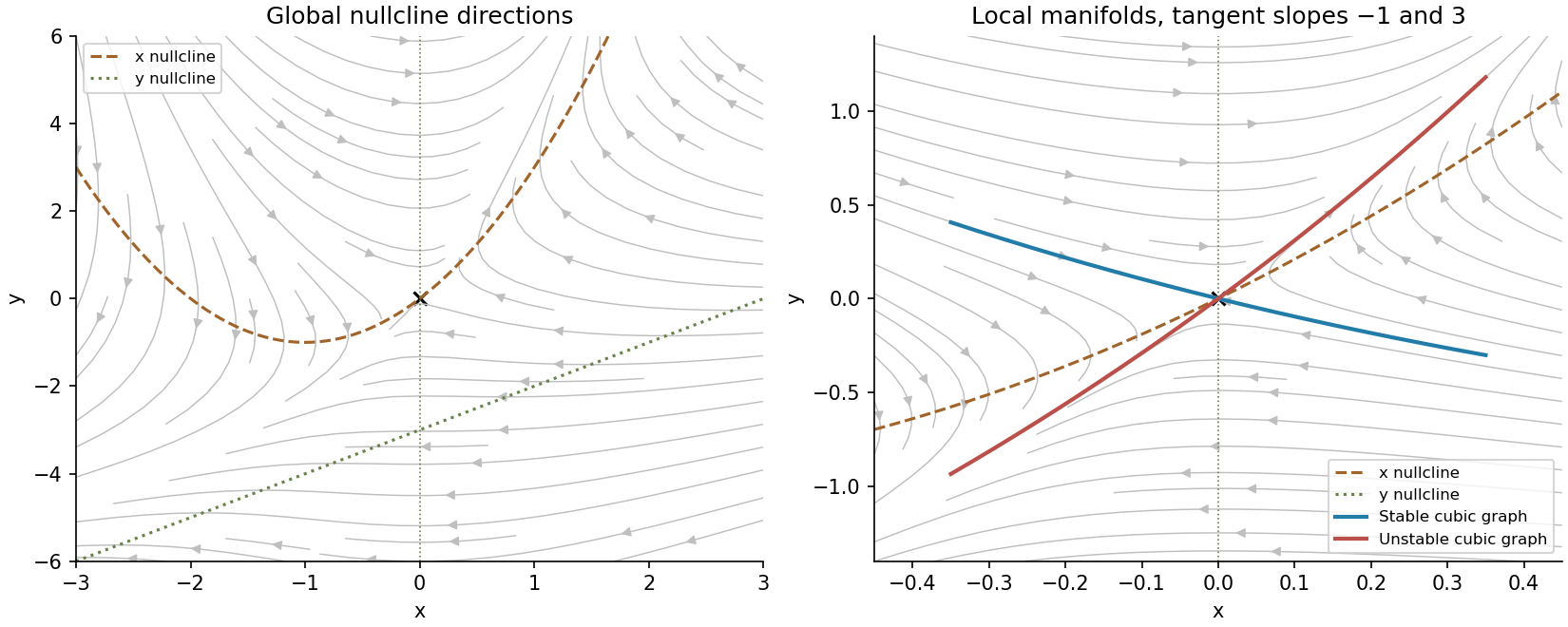
In this system, the $x$ nullcline is $y=x^2+2x$ and the $y$ nullclines are $x=0$ and $y=x-3$. Substituting the first into the second gives $x(x^2+x+3)=0$. Since the quadratic has discriminant $-11$, the origin is the only real equilibrium. Its Jacobian matrix $\left(\begin{array}{cc}-2& 1\\ 3& 0\end{array}\right)$ has eigenvalues $-3,1$, with eigenvectors $(1,-1)$ and $(1,3)$. It is therefore a hyperbolic saddle.

Set $y=h(x)$ for either manifold. Invariance requiresFor $h=sx+b{x}^2+c{x}^3+O(x^4)$, matching the linear coefficient gives $s=-1$ or $s=3$. The quadratic and cubic coefficients respectively satisfyFor the stable slope $s=-1$, this yields $b=3/7$, $c=-9/98$; for the unstable slope $s=3$, it gives $b=1$, $c=1/6$. ThusSubstituting back into $\dot{x}$ gives the reduced dynamicsThe signs of the linear terms confirm attraction and repulsion along the respective curves.

In the phase portrait, $\dot{x}$ is positive above its parabolic nullcline and negative below it; $\dot{y}$ has sign $x(3+y-x)$. The stable branches approach the saddle and the unstable branches leave it in opposite directions. There can be no periodic orbit, since such an orbit would require total enclosed equilibrium index $+1$, while the only equilibrium has index $-1$. There is no homoclinic excursion either: eliminating $y$ gives $\ddot{x}+(2+x)\dot{x}=x(x^2+x+3)$, so a positive turning point is a strict local minimum and a negative one a strict local maximum. A loop returning to zero would require the opposite extremum somewhere. Hence bounded forward trajectories lie on the stable manifold and approach zero; other trajectories eventually leave compact regions, without a claimed universal rate or infinite-time existence at infinity. The figure shows the global nullclines and the local cubic manifold approximations; the latter are used only near zero.