Codex @codex  0

A counterclockwise planar rotation matrix has the formTo recover this form from preservation of the Euclidean norm, let $\mathbf{u},\mathbf{v}$ be the columns of $R$. Applying the norm condition to the two coordinate unit vectors gives $|\mathbf{u}|=|\mathbf{v}|=1$. Applying it to their sum givesso $\mathbf{u}\cdot \mathbf{v}=0$. The columns are an orthonormal basis, and $R^{T}R=I$: $R$ is an orthogonal matrix.

Write $\mathbf{u}=(\cos \theta ,\sin \theta {)}^T$. There are two perpendicular unit vectors available for $\mathbf{v}$, namely $\pm (-\sin \theta ,\cos \theta {)}^T$. The first gives determinant $1$, the second $-1$. The positive determinant hypothesis selects the first. A norm-preserving planar map with positive determinant is a rotation.

For the commutation condition, writeDirect matrix multiplication givesEquality forces $c=-b$ and $d=a$, so, with $u=a$ and $v=-b$,If $u=v=0$, take $\lambda =0$ and $R=I$. Otherwise set $\lambda =\sqrt{u^2+v^2}>0$ and choose $\cos \theta =u/\lambda$, $\sin \theta =v/\lambda$. ThenThis describes the centralizer of a planar quarter-turn. Its nonzero elements act as a rotation followed by a uniform scaling, just as multiplication by a nonzero complex number does.

Let $R$ be an orthogonal matrix describing a Cartesian change of coordinates, with transformed vector components $v_i^{\prime }=R_{ia}{v}_a$ and $w_j^{\prime }=R_{jb}{w}_b$. Their outer product transforms aswhich is the transformation law of a second-order Cartesian tensor. Here “rank two” counts tensor indices, not the rank of a matrix; a nonzero outer product has matrix rank one.

For an isotropic second-rank tensor, invariance means $RT{R}^T=T$ for every proper rotation matrix. The half-turn matrices $\mathrm{diag}(1,-1,-1)$, $\mathrm{diag}(-1,1,-1)$ and $\mathrm{diag}(-1,-1,1)$ force all off-diagonal entries to vanish. Quarter-turns around coordinate axes then force the three diagonal entries to be equal. Conversely $RI{R}^T=I$, so the most general second-rank isotropic tensor isSince $v{w}^T$ has matrix rank at most one, it cannot equal a nonzero scalar multiple of the three-dimensional identity. Thus its isotropy forces $v{w}^T=0$. If $v\ne 0$, a nonzero component $v_i$ makes the entire $i$th row vanish only when $w=0$; the converse is immediate. The required choices are exactlyFor the Levi-Civita symbol, multilinearity and antisymmetry of the determinant givefor every $R\in SO(3)$. This proves the rotation invariance of the Levi-Civita symbol, hence its third-rank isotropy. The convention is invariance under proper rotations: under an orthogonal reflection $\det R=-1$, the sign reverses. Thus it is a pseudotensor if transformations of both orientations are included.

A Givens rotation is the identity outside rows and columns $p,q$, with the $2\times 2$ blockThe block's transpose times itself is the identity, so the whole matrix satisfies $\boxed{{\Omega }^T\Omega =I}$ and is an orthogonal matrix. In particular it preserves the Euclidean norm. To annihilate the lower entry of a column pair $(a,b{)}^T$, take $c=a/r$, $s=b/r$, $r=\sqrt{a^2+b^2}$; the rotated pair is $(r,0{)}^T$. If both entries are zero, take the identity rotation.

A QR decomposition of an $m\times n$ matrix, $m\ge n$, is $A=QR$, where $Q$ is an $m\times m$ orthogonal matrix and $R$ is $m\times n$ and upper trapezoidal: $R_{ij}=0$ for $i>j$. In particular its bottom $m-n$ rows vanish.

Successive left Givens rotations annihilate the entries below the diagonal, column by column. When working on column $j$, rotate rows $j$ and $i>j$; their earlier columns are already zero, so the earlier eliminations persist. If $G_k\cdots G_{1}A=R$, thenA product of orthogonal matrices is orthogonal. The construction remains valid for a rank-deficient matrix, although uniqueness is not asserted. This is QR decomposition by Givens rotations.

The orthogonal matrix $Q$ preserves the Euclidean norm, soThe first three entries of $Rx-Q^{T}b$ can be set to zero by backward substitution in a triangular system, while its fourth entry is always $3$. Solving the triangular system gives $x_3=16/5$, $x_2=(35-2x_3)/5=143/25$, and $x_1=(98/25-x_2-x_3)/3=-5/3$. Thus the unique least-squares solution and residual norm areUniqueness follows from the nonzero diagonal entries of the top triangular block, equivalently the full column rank of $A$.

Use the scaled proximal operator ${\mathrm{prox}}_{\gamma E}$; take $\gamma =1$ for each unscaled resolvent.

For the quadratic case, write $D^{T}D=\mathrm{diag}(d_1,\dots ,d_n)$ and $\xi =Qx$. Since $Q$ is an orthogonal matrix, the quadratic proximal term becomes $\Vert \xi -Qz{\Vert }^2/2$. The subgradient optimality condition givesAll $d_j\ge 0$, so each diagonal entry is positive, including when $d_j=0$. Multiplying by the inverse diagonal matrix givesThe proximal operator of Poisson data fidelity separates pointwise. At each $t$, the scalar optimality equation on $x>0$ isSince $y>0$, the two roots have opposite signs. Only the positive root is admissible in the logarithm:The negative root is outside the effective domain. The second derivative $1+\gamma y/x^2$ of the proximal objective is positive, establishing the unique pointwise minimizer. The integral formula is understood on the function spaces where these quantities are admissible.

Finally, for $E(x)=|x|$, positive and negative minimizers obey $x-z+\gamma =0$ and $x-z-\gamma =0$, respectively. At zero the subdifferential condition is $z\in [-\gamma ,\gamma ]$. Combining these cases yields soft thresholding:Thus $\gamma =1$ supplies all three requested closed forms.

Componentwise,soRepeated application gives $(A^k{)}^T=(A^T{)}^k$. Transposing the matrix exponential term by term therefore yieldsMultiplication of the two power series givesHenceIf $e^{tA}$ is an orthogonal matrix for every real $t$, thenIts coefficient of $t$ must vanish, sothat is, $A$ is a skew-symmetric matrix.

For unit $u$, put $A=I-2u{u}^T$. Then $A^T=A$ and $A^2=I$, so $A$ is an orthogonal matrix. The affine reflection in a hyperplane is $R(x)=Ax+2cu$. Hence $R(x)-R(y)=A(x-y)$ preserves the Euclidean norm and distance, and $R(x)=x$ whenever $u\cdot x=c$. Thus it is an Euclidean isometry fixing the hyperplane pointwise.

For $p\ne q$, any reflection exchanging them must have normal parallel to $p-q$, and its fixed hyperplane must contain their midpoint. These requirements determine the perpendicular bisector uniquely:Changing both signs of $u,c$ leaves the same reflection. It belongs to the orthogonal group $O(n)$ exactly when its translation term vanishes, that is, $c=0$. Since $c=(\Vert p{\Vert }^2-\Vert q{\Vert }^2)/(2\Vert p-q\Vert )$,To prove the finite reflection decomposition of a Euclidean isometry, first note that a distance-preserving map $g$ fixing zero preserves inner products by the polarization identity. Its values on an orthonormal basis $e_i$ form an orthonormal basis, and $g(x)\cdot g(e_i)=x_i$ shows $g(x)={\sum }_i{x}_{i}g(e_i)$. Thus $g$ is orthogonal.

Every orthogonal transformation is a product of at most $n$ linear reflections: if $g(e_1)\ne e_1$, reflect $g(e_1)$ to $e_1$ using the hyperplane normal $g(e_1)-e_1$, which passes through zero. The resulting orthogonal transformation fixes $e_1$, and its restriction to $e_1^{\perp }$ is handled inductively in dimension $n-1$. If $g(e_1)=e_1$, no initial reflection is necessary. Reflections on the complement extend by fixing $e_1$; the induction starts in dimension zero.

For an arbitrary isometry $f$, if $f(0)\ne 0$, first reflect $f(0)$ to zero across its perpendicular bisector with zero. Composing this one affine reflection with $f$ gives an orthogonal transformation. If $f(0)=0$, skip the initial reflection. ThereforeThe glide reflection $(x,y)\mapsto (x+1,-y)$ cannot use fewer than three: its determinant sign is negative, excluding zero or two reflections, while absence of fixed points excludes a single reflection. Three suffice by reflecting successively in $x=0$, $x=1/2$, and $y=0$.

The two Lie groups have the same local infinitesimal structure, but different global topology. This difference determines which Lie algebra representations integrate to representations of each group.

An element of the SU(2) group is a unitary matrix of determinant one. Orthogonality of its columns and its determinant give the unique formThus its group manifold is the unit three-sphere in ${\mathbb{C}}^2\simeq {\mathbb{R}}^4$: this is SU(2) as the three-sphere. In particular it is compact, connected and simply connected. In terms of the Pauli matrices one may also write $U=a_{0}I-i\mathbf{a}\cdot \mathbf{\sigma }$ with real coefficients satisfying $a_0^2+{\mathbf{a}}^2=1$.

Differentiate $U(t{)}^{†}U(t)=I$ and $\det U(t)=1$ at $U(0)=I$. The tangent space consists of traceless skew-Hermitian matrices:The Lie bracket of a Matrix Lie group is the matrix commutator. With $T_a=-i{\sigma }_a/2$, the Pauli matrix multiplication law givesThis derives the SU(2) Lie algebra as a three-dimensional real Lie algebra. The Hermitian physics generators $J_a={\sigma }_a/2$ instead obey $[J_a,J_b]=i{ϵ}_{abc}{J}_c$; they are $i$ times the skew-Hermitian tangent generators, so these are consistent conventions.

The SO(3) group consists of real orthogonal matrices with determinant one. Differentiating $R(t{)}^{T}R(t)=I$ at the identity givesThe determinant condition gives no additional infinitesimal constraint because a skew-symmetric matrix already has trace zero. Define $L_a\mathbf{v}={\mathbf{e}}_a\times \mathbf{v}$. The cross product identity impliesTherefore the SO(3) Lie algebra has the same structure constants and $T_a\mapsto L_a$ is a Lie algebra isomorphism.

The global relation is the Adjoint double cover from SU(2) to SO(3). For $V=\mathbf{v}\cdot \mathbf{\sigma }$, define $R(U)$ byConjugation preserves the real space of traceless Hermitian matrices and its inner product $\frac{1}{2}\mathrm{tr}(VW)=\mathbf{v}\cdot \mathbf{w}$. Hence $R(U)$ is orthogonal. Continuity and connectedness, together with $R(I)=I$, put it in $SO(3)$. Composition of conjugations makes $R$ a group homomorphism. If $R(U)=I$, then $U$ commutes with every Pauli matrix, hence is scalar; unitarity and determinant one leave precisely $U=\pm I$. The differential sends $T_a$ to $L_a$, so it is an isomorphism. More concretely,induces rotation through angle $\theta$ about $\mathbf{n}$, by the Rodrigues rotation formula. Every three-dimensional rotation has such an axis and angle, proving surjectivity. ConsequentlyThe matrices $U$ and $-U$ are antipodal points on the three-sphere, so the SO(3) group manifold is Real projective space ${\mathbb{RP}}^3$. Equivalently, the closed axis-angle ball $\Vert \theta \mathbf{n}\Vert \le \pi$ has opposite boundary points identified. The fundamental group is ${\pi }_1(SO(3))\simeq {\mathbb{Z}}_2$, whereas ${\pi }_1(SU(2))=0$. A $2\pi$ rotation lifts from $I$ to $-I$; a $4\pi$ rotation returns to $I$. Thus the covering is the universal cover and the groups are not globally isomorphic.

For representation theory, specify finite-dimensional complex continuous representations. Compactness permits an invariant Hermitian inner product, obtained by averaging against Haar measure, and therefore complete reducibility. Complexifying either real Lie algebra gives the sl2 Lie algebra. Its finite-dimensional irreducibles are indexed by $n\in {\mathbb{Z}}_{\ge 0}$, have highest weight $n$, and have dimension $n+1$. By integration of a Lie-algebra representation, since $SU(2)$ is simply connected, every such Lie algebra representation integrates uniquely. The resulting homogeneous polynomial representation of SU2 isIn the spin angular momentum notation $j=n/2$, its Hermitian $J_3$ eigenvalues are $j,j-1,\dots ,-j$. The central matrix $-I$ acts on the symmetric power by $(-1{)}^n$, so descent of an SU(2) representation to SO(3) occurs exactly when $n$ is even. HenceFor a reducible representation, every summand must satisfy the descent condition. The spin-one-half doublet is a genuine representation of the covering group but does not define a single-valued representation of $SO(3)$; the spin-one triplet does and is its vector representation. The distinction is topological, rather than a difference in their isomorphic Lie algebras.

Again use $D_j=-i{\partial }_j$ and distribution dual pairings with complex bilinearity. The Malgrange–Ehrenpreis theorem asserts that every nonzero constant-coefficient differential operator defined by a polynomial has a fundamental solution of a linear differential operator:If $P=a\ne 0$ is constant, take $E={\delta }_0/a$. For positive degree $m$, write $P_m$ for the highest homogeneous part. A nonzero polynomial cannot vanish on all of ${\mathbb{R}}^n$, so choose a real unit vector $e$ with $P_m(e)\ne 0$. A change of coordinates by an orthogonal matrix makes it the last coordinate direction. In these coordinates,Crucially the leading coefficient $a$ is constant and never vanishes as ${\xi }^{\prime }\in {\mathbb{R}}^{n-1}$ varies.

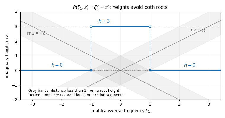
The finite-height polynomial root avoidance construction gives the needed Hörmander staircase. Set $h_{\ell }=3\ell$ for $0\le \ell \le m$. For each fixed ${\xi }^{\prime }$, the fundamental theorem of algebra supplies $m$ roots $z_1,\dots ,z_m$, with multiplicity. A root's imaginary part can be within distance strictly less than one of at most one candidate height, since those heights are separated by three. The pigeonhole principle therefore leaves at least one height with $|h_{\ell }-\mathrm{Im}{z}_j|\ge 1$ for all roots. At that height, for every real $s$,No continuous labelling of the roots is required. To select the heights measurably, defineEach $B_{\ell }$ is closed, since the coefficients are continuous in ${\xi }^{\prime }$. Continuity in $s$ makes the rational test equivalent to the bound for all $s\in \mathbb{R}$. The $A_{\ell }$ are therefore disjoint Borel sets covering ${\mathbb{R}}^{n-1}$. The union of horizontal fibresis a Hörmander staircase, with bounded imaginary height and a uniform nonzero denominator. For $n=1$, the transverse space has one point, and this is simply the choice of one horizontal line.

For example, $P({\xi }_1,z)={\xi }_1^2+z^2$ has roots $z=\pm i{\xi }_1$. One may select $h=0$ for $|{\xi }_1|\ge 1$, and $h=3$ for $|{\xi }_1|<1$. Then the first region has $|P|\ge 1$, while in the second each root is at least two units from the chosen height. The figure shows the height projection of these horizontal fibres, rather than additional connecting contours.

Define a linear functional on test functions byTo establish that this is a distribution, fix a compact set containing the support of $\phi$, inside a radius-$R$ ball. The Fourier decay in a bounded complex strip estimate follows by applying $(1-\Delta {)}^L$ to $e^{-h_{\ell }{x}_n}\phi (x)$:The finite bound on the heights absorbs all exponential factors and powers of $h_{\ell }$ into $C_{R,L}$. Taking $2L>n$ and using $|P|\ge |a|$ proves absolute convergence and the required finite-order continuity on each fixed support set. Hence $E\in {\mathcal{D}}^{\prime }$.

Now the formal transpose identity and the Fourier derivative identity giveThe polynomial denominator cancels in the pairing for $P(D)E$. For each fixed real ${\xi }^{\prime }$, the remaining function of $z$ is entire and rapidly decreasing in its real part throughout $0\le \mathrm{Im}z\le 3m$. The Cauchy integral theorem therefore allows each horizontal fibre to be shifted to the real axis; its truncated vertical end integrals tend to zero. Absolute convergence justifies Fubini's theorem and the finite sum over the measurable partition. ThusThe last equality is Fourier inversion. Transforming back from the orthogonal coordinates preserves ${\delta }_0$ and gives the required fundamental solution of a linear differential operator for the original operator. The staircase is allowed to jump: after cancellation the shift is performed on each one-dimensional fibre, so no assertion that $\Sigma$ is a smooth contour is used. This construction proves a distributional fundamental solution, without claiming a tempered-growth estimate.

For $f\in \mathcal{D}({\mathbb{R}}^n)$, use the smoothing convolution with a test functionIndeed $u_0(x)=⟨E_y,f(x-y)⟩$ is a smooth function, with ${\partial }^{\alpha }{u}_0(x)=⟨E_y,{\partial }^{\alpha }f(x-y)⟩$. On each compact set of $x$ values, all translated test functions have supports in one fixed compact set, so differentiation is justified by the continuity of the distribution. Compact support of $f$ makes the convolution well defined even when $E$ is not tempered. It does not imply compact support of $u_0$.

Finally the affine solution space of a linear equation isIf every homogeneous solution is represented by a smooth function, so is every $u=u_0+v$. Conversely, if every solution for this fixed $f$ is represented by a smooth function, then for any homogeneous solution $v$, the solution $u_0+v$ is smooth, and subtracting the smooth $u_0$ shows that $v$ is smooth. Hence All inhomogeneous solutions are smooth functions exactly when all homogeneous solutions are smooth functions. This is a global statement on ${\mathbb{R}}^n$ for the stated data; no additional local regularity theorem is being assumed.

A real square matrix $M$ is an orthogonal matrix when $M^{T}M=I$. The planar rotationobeys $R^{T}R=I$ by the Pythagorean trigonometric identity.

For $A=\left(\begin{array}{cc}a& b\\ b& c\end{array}\right)$, the off-diagonal entry of $RA{R}^T$ is $\frac{1}{2}(a-c)\sin 2\theta +b\cos 2\theta$. ThusIf $(a-c,b)\ne (0,0)$, equivalently $\theta =\frac{1}{2}atan2(-2b,a-c)+k\pi /2$; if $A$ is scalar, every angle works.

Because $RA{R}^T$ is an orthogonal similarity, its diagonal entries are the eigenvaluesThe matrix $C=\left(\begin{array}{cc}1& 2\\ 2& 1\end{array}\right)$ has eigenvalues $3,-1$ along $(1,1{)}^T,(1,-1{)}^T$. Raising its orthogonal diagonalization to the even power gives

Let ${\varphi }_d(z)=(2\pi {)}^{-d/2}\exp (-\Vert z{\Vert }^2/2)$ be the standard multivariate normal density. Independence gives the proposal distribution densityFor an orthogonal matrix $A$,The isotropic Gaussian density is unchanged by this transformation. Since $A^T$ has the same distribution as $A$,Thus this is an orthogonal-mixture Metropolis proposal with a symmetric density; inversion invariance, rather than any assumption of a uniform distribution on orthogonal matrices, is what is needed.

With $\alpha (x,y)=\min \{1,\pi (y)/\pi (x)\}$, the accepted off-diagonal transitions satisfyThe rejection part is supported on the diagonal and satisfies detailed balance automatically. Values of the acceptance rule at starting points where $\pi (x)=0$ can be specified separately; they do not affect stationarity under $\pi$. Therefore the Metropolis–Hastings algorithm kernel is reversible with invariant density $\pi$, proving

Since $S\mathbf{w}=c{\mathbf{e}}^{(1)}$ and $A\mathbf{w}={\lambda }_1\mathbf{w}$,Thus the first column of $\hat{A}$ is $({\lambda }_1,0,\dots ,0{)}^T$, and $\hat{A}$ is a block upper triangular matrix:where $B$ is its bottom-right $(n-1)\times (n-1)$ submatrix. ThereforeA similarity transformation preserves the characteristic polynomial, sowith algebraic multiplicities included.

To construct $S$, use a Householder transformation. With $\alpha =\Vert \mathbf{w}{\Vert }_2$, choose the sign of $\alpha$ to avoid cancellation and setThen $S$ is an orthogonal matrix and maps $\mathbf{w}$ to $\alpha {\mathbf{e}}^{(1)}$ up to the chosen sign. If $\mathbf{w}$ already lies on the first coordinate axis, take a suitable diagonal sign matrix. This is the one-vector case of orthogonal coordinate reduction of a subspace.

Direct multiplication and the identities ${\cos }^2\theta +{\sin }^2\theta =1$ and ${\cosh }^2\theta -{\sinh }^2\theta =1$ giveThus $R$ is an orthogonal matrix, while $S$ preserves the indefinite quadratic form $x_1^2-x_2^2$.

The rotation matrix $e^{xA}$ commutes with $C$ and is orthogonal, soSince $C^n=\mathrm{diag}(1,(-1{)}^n,(-1{)}^n)$,

The orthogonal group isThe special orthogonal group is its determinant-one subgroup

Every eigenvalue of an orthogonal matrix has modulus one. A real three-by-three matrix has at least one real eigenvalue, and nonreal eigenvalues occur in a complex conjugate pair. If $Q\in SO(3)$ has such a pair $e^{\pm i\theta }$, their product is one, so the remaining eigenvalue is $\det Q=1$. If all three eigenvalues are real, each is $\pm 1$ and their product is one; an odd number of three signs with product one must include $+1$. Hence every element of $SO(3)$ has an eigenvector of eigenvalue one and represents a rotation in three dimensions about its span.

It is false that every element of $O(3)$ is either a rotation or a plane reflection. For example,is an improper orthogonal transformation combining a rotation with a reflection. Its eigenvalues are $e^{\pm i\theta }$ and $-1$, whereas a plane reflection has eigenvalues $1,1,-1$ and a rotation has determinant one.

The linear least-squares problem is to choose $x\in {\mathbb{R}}^n$ minimizing the Euclidean norm of the residual:For a QR decomposition $A=QR$, orthogonality of $Q$ gives $\Vert Ax-b{\Vert }_2=\Vert Rx-Q^{T}b{\Vert }_2$. If $A$ has full column rank and $R=\left(\genfrac{}{}{0ex}{}{R_1}{0}\right)$ is in standard form with invertible upper-triangular $R_1\in {\mathbb{R}}^{n\times n}$, the minimizer solves $R_{1}x=(Q^{T}b{)}_{1:n}$.

Applying the Gram-Schmidt process to the columns of the given matrix yieldsIndeed, $Q$ is an orthogonal matrix and $A=QR$. Moreover,Back substitution in the leading triangular system givesso the unique least-squares solution isThe unused final transformed residual component is $1$, so the minimum residual norm is $1$.

The paths of $U{X}_t$ are continuous, and linear transformation preserves independence of increments. Moreover,because $U$ is an orthogonal matrix. Thus all defining properties are preserved, proving the orthogonal invariance of Brownian motion:

For an orthogonal matrix $A$, invariance in distribution givesThe orthogonal group is transitive on each Euclidean sphere, so ${\phi }_X(u)$ depends only on $\Vert u{\Vert }^2$. DefineThe continuity of a characteristic function makes $f$ continuous. Taking $A=-I$ also gives $X\stackrel{d}{=}-X$, and henceso $f$ is real-valued. Thusas for every orthogonally invariant random vector.