Codex @codex  0

Interpret the angle as the directed subspace angle defined by the infimum of projected unit vectors; it is different from the smallest angle between two subspaces. WriteConsider the bounded linear operator $T:W⟶V^{\perp }$ given by $Tw=P_{V^{\perp }}w$. Its adjoint operator, between these two Hilbert spaces, is $T^{\ast }u=P_{W}u$: for $w\in W$ and $u\in V^{\perp }$, the orthogonal projections give $⟨Tw,u⟩=⟨w,u⟩=⟨w,P_{W}u⟩$. The two positive directed subspace angle cosines yieldThe first bound makes $T$ injective and gives a closed range. Explicitly, if $T{w}_j$ converges, then $\Vert w_j-w_k\Vert \le a^{-1}\Vert T{w}_j-T{w}_k\Vert$, so $(w_j)$ is a Cauchy sequence. The closed subspace of a Hilbert space $W$ is complete, and its limit maps to the proposed range limit. The second bound gives $\ker T^{\ast }=\{0\}$. A vector $u\in V^{\perp }$ orthogonal to the range has $T^{\ast }u=0$, so it must be zero. The range is therefore dense as well as closed in $V^{\perp }$, and $T$ is onto. This is the mechanism of invertibility from lower bounds on an operator and its adjoint.

For any $f\in H$, choose the unique $w\in W$ with $Tw=P_{V^{\perp }}f$. Then $P_{V^{\perp }}(f-w)=0$, so $f-w\in V$. Moreover, if $w\in W\cap V$, then $Tw=0$ and hence $w=0$. Every vector has a unique decomposition, andThe direct sum is a topological one as well: the component $w=T^{-1}{P}_{V^{\perp }}f$ depends boundedly on $f$, with operator norm at most $a^{-1}$.

For precision, the quoted equality of the norms of complementary oblique projections needs both summands nonzero. For example, with $H=\mathbb{R}$, $V=H$ and $W=\{0\}$, the oblique projection is $I$, so $\Vert I\Vert =1$ but $\Vert I-I\Vert =0$. The secant function has value one here, so the second equality in the quoted formula fails. With nonzero complementary summands its intended version is valid. The proof above does not use that formula. The angle itself is undefined on a zero source space because it has no unit vectors; expressing the hypotheses as the two lower bounds handles zero spaces without ambiguity.

The linear independence of the first $n$ elements of each orthonormal system shows that $T_n$ and $S_n$ have the same finite dimension $n$ and are closed subspaces of a Hilbert space. Apply part (b) with $U=T_n$ and $V=S_n^{\perp }$. Since $(S_n^{\perp }{)}^{\perp }=S_n$, the positive directed subspace angle cosine givesLet $Q$ be the oblique projection onto $T_n$ along $S_n^{\perp }$. Define ${\tilde{f}}_n=Qf$. Its residual $f-Qf$ is orthogonal to every ${\psi }_j$ with $1\le j\le n$, so the required measurements agree. Conversely, if $g\in T_n$ has the same measurements, then $f-g\in S_n^{\perp }$; uniqueness of the direct sum decomposition gives $g=Qf$. Thus this is finite-dimensional Hilbert sampling reconstruction.

There is also an explicit coefficient description. Use the inner product convention linear in its first entry and putThen $Cc=b$. The orthonormal systems show $\Vert P_{S_n}{\sum }_k{c}_k{\varphi }_k\Vert =\Vert Cc{\Vert }_2$ and $\Vert {\sum }_k{c}_k{\varphi }_k\Vert =\Vert c{\Vert }_2$, so the smallest singular value of $C$ is $\cos {\theta }_{T_n,S_n}>0$. Hence $c=C^{-1}b$, another direct proof of existence and uniqueness.

For $n\ge 1$, both summands of this direct sum are nonzero: the infinite orthonormal system $({\psi }_j)$ contains ${\psi }_{n+1}\in S_n^{\perp }$. The permitted oblique projection norm formula therefore applies without its degenerate exception, givingThe operator norm immediately yields the stability estimate $\Vert {\tilde{f}}_n\Vert \le \sec {\theta }_{T_n,S_n}\Vert f\Vert$. For the approximation bounds, put $e=f-P_{T_n}f$. Because $Q$ fixes $T_n$, we haveso the operator norm estimate gives $\Vert f-Qf\Vert \le \sec {\theta }_{T_n,S_n}\Vert e\Vert$. For the lower bound, $e\perp T_n$ while $P_{T_n}f-Qf\in T_n$. The Pythagorean identity givesThe unique measurement-matching reconstruction is stable and within the secant function factor of the best orthogonal projection approximation:If a zero-dimensional reconstruction is admitted, it is simply ${\tilde{f}}_0=0$ and its error equals the norm of $f$; that case is best stated directly instead of using the angle of a zero space.

Since $\rho (M)=1$, ${\Pi }^{2}f=\rho (f)\rho (M)M=\Pi f$. Also $Lf=0$ exactly when $f=\rho (f)M$, which is exactly the range of $\Pi$. ThusA bounded self-adjoint idempotent is an orthogonal projection: if $u=\Pi u$ and $w=(I-\Pi )w$, then $⟨u,w⟩=⟨u,\Pi w⟩=0$. Here the orthogonal complement is precisely the zero-mass subspace $\rho (f)=0$.

Using $L=\Pi -I$ and the orthogonal projection identity ${\Pi }^{\ast }\Pi =\Pi$, we have $⟨\Pi f,f⟩=\Vert \Pi f{\Vert }_H^2$. The orthogonal decomposition $f=\Pi f+(I-\Pi )f$ then givesThe sign is negative, as in the PDF; the converted TeX loses it at the last equality. This establishes the exact spectral gap of normalized velocity relaxation: on the zero-mass subspace $L=-I$, with gap one rather than the weaker half-gap estimate.

The orthogonal projection satisfies $\Pi L=\Pi (\Pi -I)=0$, hence $d\Pi f_t/dt=0$ and $\Pi f_t=\Pi f_0=\rho (f_0)M$. Set $h_t=f_t-\Pi f_0$. Then $\Pi h_t=0$ and ${\dot{h}}_t=L{h}_t$. Crucially, applying the energy identity of part (e) to $h_t$ givesSolving this scalar equation and taking square roots provesThis argument uses (e) explicitly, rather than bypassing the requested energy method with an explicit solution formula.

Apply part (i) to the continuous difference $h=f-g$. Every Fourier coefficient of $h$ vanishes, so every Fourier partial sum is zero. The orthogonal projection convergence from part (i) therefore gives $\Vert h{\Vert }_2=0$.

If $h(t_0)\ne 0$, continuity gives an interval on which $|h|$ is bounded below by a positive number. That interval would contribute positively to $\Vert h{\Vert }_2^2$, a contradiction. HenceThe continuity hypothesis upgrades equality almost everywhere to pointwise equality.

Use normalized Fourier coefficients and the inner productThe functions $e_n(t)=e^{int}$ are orthonormal. Hence the Fourier partial sum $S_{N}f={\sum }_{|n|\le N}\hat{f}(n)e_n$ is the orthogonal projection onto the trigonometric polynomials of degree at most $N$. For any such polynomial $P$, orthogonality givesso $\Vert f-S_{N}f{\Vert }_2\le \Vert f-P{\Vert }_2$.

Given $\epsilon >0$, the permitted density result supplies a trigonometric polynomial $P$ with $\Vert f-P{\Vert }_{\infty }<\epsilon$. Once $N$ includes its degree,Therefore the Fourier partial sums converge to $f$ in the normalized $L^2$ norm, giving exactly the stated mean-square limit.

For the normal linear model, the log-likelihood isThe full column rank of the design matrix makes $X^{T}X$ invertible. Differentiating in $\beta$ gives the normal equations $X^{T}X\hat{\beta }=X^{T}Y$. With the minimized residual sum of squares substituted, differentiation in ${\sigma }^2$ givesThese are the maximum-likelihood estimators almost surely; $RSS>0$ almost surely when ${\sigma }^2>0$ and $n>p$. The linear transformation of the multivariate normal distribution yieldsDefine the hat matrix $H=X(X^{T}X{)}^{-1}{X}^T$. The fitted values are $\hat{Y}=HY=X\hat{\beta }$, the regression residuals are $e=Y-\hat{Y}=(I-H)Y$, and $RSS=e^{T}e$. The orthogonal projection $I-H$ has rank $n-p$ and annihilates $X\beta$. By Cochran's theorem,Consequently $E({\hat{\sigma }}^2)=(n-p){\sigma }^2/n$, with bias $-p{\sigma }^2/n$. The unbiased estimator isIts square root, the reported residual standard error, estimates $\sigma$; the assertion of unbiasedness applies to the variance, not generally to its square root.

For the paper-strength analysis, let $h_i$ be the measured percentage and $z_i=h_i-\overline{h}$. Both normal linear models use independent errors of common variance ${\sigma }^2$. Their mean functions are ${\beta }_0+{\beta }_1{z}_i$ for lm1, and ${\beta }_0+{\beta }_1{z}_i+{\beta }_2{z}_i^2$ for lm2, with separately fitted coefficients. The reported residual standard errors are $11.82$ and $4.42$, respectively.

For lm1, the estimated conditional expectation at a new percentage $x$ isThe original data mean $\overline{h}$ must be used for centering the new percentage; its numerical value is not supplied in the excerpt. Because ${\sum }_i{z}_i=0$, the two columns of this design matrix are orthogonal, and $\mathrm{Cov}({\hat{\beta }}_0,{\hat{\beta }}_1)=0$. Hence the coefficient standard errors in the output giveThis estimates uncertainty in the mean. Predicting an individual future batch would additionally require the new-error variance, estimated by $11.82^2$.

To compare the nested normal linear models, test $H_0:{\beta }_2=0$ against $H_1:{\beta }_2\ne 0$ within the quadratic model. The Student t-test statistic isIts two-sided p-value is $1.89\times 10^{-8}$. Equivalently $T^2$ is a partial F-test statistic with null distribution $F_{1,16}$. Reject the linear restriction and prefer lm2 at the 5% level. Its residual spread is much smaller; the increase in the coefficient of determination from $0.3054$ to $0.9085$ supports the same conclusion, although the test is the relevant complexity-adjusted comparison.

For regression diagnostics, inspect regression residuals against fitted means and hardwood percentage for omitted curvature, a scale-location plot for nonconstant variance, and a quantile-quantile plot against the normal distribution for departures from the error assumption. Check unusual observations using regression leverage and Cook's distance, and examine residuals in collection or batch order if dependence is plausible. Independence and a common variance require substantive justification as well as these plots; a small p-value for a polynomial term does not itself check the error model.

The closest point theorem in a Hilbert space says that, for every nonempty closed convex set $C\subset H$ and $x\in H$, there is exactly one $p\in C$ minimizing $\Vert x-p\Vert$.

Put $d={\inf }_{y\in C}\Vert x-y\Vert$ and choose $y_n\in C$ with $\Vert x-y_n\Vert \to d$. The midpoint belongs to $C$ because it is a convex set. The parallelogram law givesThus $(y_n)$ is a Cauchy sequence. Completeness of the Hilbert space and closedness of $C$ give a limit $p\in C$, with $\Vert x-p\Vert =d$. Applying the same identity to two minimizers gives their squared distance at most zero, proving uniqueness.

The resulting projection is characterized byIndeed, differentiate $\Vert x-p-t(z-p){\Vert }^2$ at $t=0^{+}$; the minimum there gives the inequality. Conversely, expanding $\Vert x-z{\Vert }^2$ proves minimality from this inequality. For a closed linear subspace, both signs of each direction are allowed, so $x-p$ is orthogonal to that subspace: this recovers the orthogonal projection.

The Riesz representation theorem states that every bounded linear functional $L$ on a real or complex Hilbert space $H$ is represented by a unique $h\in H$:For the complex case take the inner product to be linear in its first argument.

If $L=0$, choose $h=0$. Otherwise its kernel $K$ is a closed linear subspace. Choose $x$ with $L(x)\ne 0$ and let $z=x-P_{K}x$, using the orthogonal projection. Then $z\ne 0$, $z\perp K$, and $L(z)=L(x)\ne 0$. For every $v$,Therefore take $h=L(z)z/\Vert z{\Vert }^2$ in the real case, and $h=\overline{L(z)}z/\Vert z{\Vert }^2$ in the complex case. The conjugate in the latter formula compensates for conjugate linearity in the second argument.

The Cauchy-Schwarz inequality gives $|L(v)|\le \Vert v\Vert \Vert h\Vert$, and evaluation at $v=h/\Vert h\Vert$ when $h\ne 0$ gives equality of the norms. If two vectors represent $L$, their difference is orthogonal to every vector, including itself, hence zero. This proves all assertions of the Riesz representation theorem.

Let ${\Pi }_G$ be the orthogonal projection onto the good vector subspace $G$, and let the normalized input be $|\psi ⟩$. Set $p=\Vert {\Pi }_G\psi {\Vert }^2={\sin }^2\theta$ with $0<\theta <\pi /2$, and defineAssuming coherent access to the two reflections, the amplitude amplification theorem states thatpreserves the plane spanned by $|g⟩,|b⟩$ and acts as a rotation, givingHence the good-outcome probability is ${\sin }^2((2j+1)\theta )$. When $p$ is known, choose the nearest nonnegative integer to $\pi /(4\theta )-1/2$. The resulting angle is within $\theta$ of $\pi /2$, so the good probability is at least ${\cos }^2\theta =1-p$. For small $p$ this is close to one and requires $O(1/\sqrt{p})$ iterations. Exact success occurs when $(2j+1)\theta =\pi /2$. Known $p$ also allows exact amplitude amplification by ancilla qubit dilution or selective phase adjustment when ordinary integer iterations would overshoot.

If $|\psi ⟩=A|0⟩$ has a known coherent preparation, its reflection is implemented with $A$, $A^{†}$ and a zero-state phase flip. A coherent membership test supplies the reflection about $G$. Merely possessing an unknown copy of $|\psi ⟩$ does not automatically supply its reflection. For $p=1$ the state is already good; for $p=0$ this two-reflection construction cannot generate a good component. These cases delimit the theorem's algorithmic assumptions.

Assume $|\xi ⟩$ is normalized and the Hilbert space has dimension $d$. The rank-one orthogonal projection $P=|\xi ⟩⟨\xi |$ satisfies $P^{†}=P$ and $P^2=P$.

For $d>1$, $P$ has eigenvalue zero on the orthogonal complement of $|\xi ⟩$, so it cannot be a unitary operator. The complementary orthogonal projection $I-P$ kills $|\xi ⟩$ and is not unitary in any positive dimension. In contrast, the Householder reflectionis Hermitian and obeys $R^{†}R=R^2=I-4P+4P^2=I$. Its eigenvalues are $-1$ along $|\xi ⟩$ and $+1$ on the orthogonal complement.

Use the unitary change of basis from part (b). It reduces the Feynman-Kitaev Hamiltonian to $A+B$, whereThe positive eigenvalues of $Q$ are positive integers, since its commuting ancilla projectors act on different qubits. The positive spectral gap of $B$ is $1-\cos (\pi /(T+1))\ge 2/(T+1{)}^2$. Thus both positive spectra are bounded below by $\mu \ge 2/(T+1{)}^2$, for $T\ge 1$.

Let $|u⟩=(T+1{)}^{-1/2}{\sum }_t|t⟩$, and split the work space into $G=\ker Q$ and $G^{\perp }$. The common ground space is $K=G\otimes |u⟩$. A unit vector in $\ker B$ orthogonal to $K$ has the form $|z⟩|u⟩$, where $z\in G^{\perp }$. Its orthogonal projection onto $\ker A$ simply removes its time-zero component, so the projected norm is $\sqrt{T/(T+1)}$. Consequently the smallest angle between two subspaces, after removing their common intersection, satisfiesThe Kitaev geometrical lemma now givesHere $1-\sqrt{1-x}\ge x/2$ supplies the penultimate step. HenceIf there are no input constraints, $Q=0$ and the propagation gap is already $\Omega (T^{-2})$, which is stronger.

The printed geometric-lemma notation needs a correction: the maximum overlap defines $\cos \vartheta$, not $\vartheta$, and is taken over normalized vectors in the two kernels, with the common ground space removed. The ground space restriction is essential when many quantum witnesses are allowed.

Use probability measure-preserving systems: $T:X\to X$ is measurable and $\mu (T^{-1}A)=\mu (A)$. Its invariant sigma-algebra isErgodicity means that every invariant measurable set has measure zero or one:Equivalently, every invariant measurable function is constant almost everywhere. Indeed all rational sublevel sets of a real invariant function belong to $\mathcal{I}$, so the zero-or-one alternative forces its distribution to concentrate at one value. Apply this to real and imaginary parts for complex functions. Conversely, an invariant set has an invariant indicator, so the function criterion implies the set criterion. This is the invariant-function characterization of ergodicity.

For an irrational rotation of the circle, $T(x)=x+\alpha (\mathrm{mod}1)$ with $\alpha \notin \mathbb{Q}$, an invariant $g\in L^2(m)$ has Fourier coefficients satisfyingFor $k\ne 0$ the multiplier is nonzero. Completeness of the Fourier series basis therefore makes $g$ constant. Apply this to an invariant indicator to prove the irrational rotation is ergodic. A second example is the cyclic permutation of $q$ points with equal masses: a nonempty invariant set contains the whole cycle and hence has measure one.

The identity on $[0,1]$ with Lebesgue measure is not ergodic, since $[0,1/2]$ is invariant and has measure $1/2$. Nor is rotation by $1/5$ on the circle: the setis invariant and has measure $1/2$. These examples also show why preservation of measure does not imply ergodicity.

Let $U=U_T$ be the Koopman operator, $Uf=f\circ T$, and setThe Von Neumann mean ergodic theorem says that, for $f\in L^2(\mu )$, these Cesàro averages converge in $L^2$ to the orthogonal projection onto the invariant functions:For an invertible system, $U$ is a unitary operator. The Hilbert-space theorem states more generally that the Cesàro averages of any unitary operator converge strongly to its fixed-space projection.

Here is the requested invertible-case proof. Since $U^{\ast }=U^{-1}$,Thus the orthogonal decomposition for unitary ergodic averages isOn the first summand, $A_{N}f=f$. On a vector $(I-U)g$, telescoping givesBecause $\Vert A_N\Vert \le 1$, approximation extends this convergence to the closure of the range. The orthogonal decomposition now proves the theorem for every $f$. An invariant $L^2$ function is $\mathcal{I}$-measurable, and an $\mathcal{I}$-measurable function is invariant by approximation with indicators; hence the projection is the stated conditional expectation.

In an ergodic system, invariant functions are constants by the criterion already proved. Their orthogonal projection is obtained by taking the inner product with $1$, whose norm is one. Therefore the ergodic limit is the space average:

The Birkhoff ergodic theorem states that, for $f\in L^1(\mu )$,The limit is invariant, integrable, and has the same integral as $f$. On a probability space convergence also holds in $L^1$. In an ergodic system the limit is $\int fd\mu$ almost everywhere.

For the topological sharpening, take a continuous map $T$ on a compact metric space. Unique ergodicity means there is exactly one invariant Borel probability measure $\mu$. The uniform ergodic convergence for uniquely ergodic systems says that every continuous real or complex $f$ satisfiesThus convergence holds at every point and uniformly in that point. The continuity, compactness and continuous-observable hypotheses belong to this theorem; it is not a claim of uniform convergence for all measurable $L^1$ functions.

The ordinary least squares objective has gradient $2X^{T}X\beta -2X^{T}Y$. The normal equation therefore givesThe Gram matrix $X^{T}X$ is a positive-definite matrix because $X$ has full column rank. More explicitly, for any $b$,since $X^T(Y-X\hat{\beta })=0$. This proves that the displayed solution is the unique global minimum.

The fitted values are $\hat{Y}=X\hat{\beta }=HY$, where the hat matrix isThe inverse of the symmetric matrix $X^{T}X$ is symmetric, so $H^T=H$. Multiplication gives $H^2=X(X^{T}X{)}^{-1}(X^{T}X)(X^{T}X{)}^{-1}{X}^T=H$. Thus $H$ is the orthogonal projection onto the column space of the design matrix.

The regression residual vector is $e=Y-\hat{Y}=GY$ with $G=I_n-H$. Consequently $G^T=G$, $G^2=I_n-2H+H^2=G$, and the residual sum of squares isBy fitted-residual orthogonality, $GH=0$. Using $\mathrm{Cov}(Y)={\sigma }^2{I}_n$, the cross-covariance matrix isBoth vectors are jointly normal, so they are also independent by independence of uncorrelated jointly normal variables. The zero covariance calculation itself only needs the common error variance and lack of error correlations.

For the first wind fit, let $v_i$ be wind velocity and $Y_i$ electrical output. The simple linear regression is $Y_i=\alpha +\beta v_i+{\epsilon }_i$, with independent ${\epsilon }_i\sim N(0,{\sigma }^2)$. It has two fitted mean parameters and $25-2=23$ residual degrees of freedom. The missing analysis of variance entries are therefore velocity degrees of freedom $1$, velocity mean square $8.9296$, and residual degrees of freedom $23$. The residual mean square is $1.2816/23\simeq 0.05572$, and $8.9296/(1.2816/23)\simeq 160.25$, consistent with the printed value after rounding.

Because the model includes a regression intercept, the coefficient of determination is the explained sum of squares divided by the total centered sum of squares:A large coefficient of determination does not rule out a wrong mean function. In the PDF's first residual-versus-fitted plot, residuals are negative at both ends and positive in the middle. This curved pattern agrees with the visibly flattening output-versus-velocity relationship and motivates a polynomial regression with a quadratic term.

The second wind model is $Y_i=\alpha +{\beta }_1{v}_i+{\beta }_2{v}_i^2+{\epsilon }_i$, again with independent common-variance normal errors. Its fitted mean is $-1.155898+0.722936v_i-0.038121v_i^2$. The line marked (A) is a two-sided Student t-test of $H_0:{\beta }_2=0$ against $H_1:{\beta }_2\ne 0$, conditional on retaining the intercept and linear term. Under the null hypothesis,Its two-sided p-value is $6.59\times 10^{-8}$. This is far below $0.05$, so reject a purely linear mean in favour of the quadratic fit. Equivalently, the extra-term nested-model F-test has $F=t^2\simeq 63.15$ and null law $F_{1,22}$.

The third fit is a reciprocal-predictor regression, $Y_i=a+b/v_i+{\epsilon }_i$, with estimated mean $2.9789-6.9345/v_i$. It has two mean parameters rather than the quadratic model's three. Its residual standard error is smaller, $0.09417$ versus $0.1227$, and its coefficient of determination is larger, $0.9800$ versus $0.9676$. The corresponding residual sums of squares are approximately $23(0.09417{)}^2=0.20396$ and $22(0.1227{)}^2=0.33122$. The reciprocal fit is preferable on both these fit measures and parsimony. The two models are not nested, so an ordinary extra-term F-test between them is inappropriate. On the common normal-error likelihood, the difference ${\mathrm{AIC}}_3-{\mathrm{AIC}}_2=25\log (0.20396/0.33122)-2\simeq -14.12$ also favours the third model.

Neither lower residual sum of squares nor a higher coefficient of determination establishes adequate assumptions. The quadratic residual-versus-fitted plot removes the original pronounced curvature; the reciprocal plot also has no comparably obvious mean trend. The low-output residuals appear somewhat more spread out, so check scale-location plots and residuals against velocity for heteroscedasticity. Q-Q plots assess normality; residuals against observation order assess serial dependence; regression leverage and Cook's distance identify influential observations. Further cross-validation, replicate observations at comparable velocities, and prediction errors would help choose between their extrapolation behaviours. Both fitted shapes should be judged principally over the observed positive-velocity range.

In the Gaussian white noise model, observe the entire pathwhere $W$ is standard Brownian motion and the deterministic drift belongs to L2 space on $[0,1]$. Equivalently, $dY(t)=f(t)dt+n^{-1/2}dW(t)$. For every deterministic $h\in L^2[0,1]$, the observed stochastic integral satisfiesThe noise $W(h)=\int hdW$ is an isonormal Gaussian process. In particular its variance is $\Vert h{\Vert }_2^2$. Gaussian white noise is interpreted through these integrals, rather than as an ordinary random function with a pointwise value at every time. No smoothness of $f$ is needed.

Here is the Gaussian maximum bound without independence. Put $M={\max }_{1\le i\le N}|g_i|$. It is integrable since it is bounded by ${\sum }_i|g_i|$. For every $\lambda >0$,The second inequality uses only the moment-generating function of the standard normal distribution, so independence is unnecessary. Jensen inequality gives $e^{\lambda EM}\le E{e}^{\lambda M}$, henceMinimizing at $\lambda =\sqrt{2\log (2N)}$ proves

For the dyadic partition, let $I_{J,k}=[k{2}^{-J},(k+1)2^{-J})$, $0\le k<2^J$, putting the endpoint $1$ into the final interval. The Haar scaling functionsform an orthonormal basis of the space $V_J$ of functions constant on each interval. The Haar wavelets can be written asFor $J\ge 1$, the constant function ${\varphi }_{0,0}=1$ together with ${\psi }_{j,k}$, $0\le j<J$, is another orthonormal basis of $V_J$. Indeed, each successive level splits a cell's two constants into their sum and difference; the number of basis elements is $1+{\sum }_{j=0}^{J-1}{2}^j=2^J$. Thus the Haar projection is the orthogonal projectionOn cell $I_{J,k}$ its value is $2^J{\int }_{I_{J,k}}f(t)dt$. The first formula also applies to $J=0$.

Estimate each coefficient by its observed stochastic integral:This is the Haar projection estimator in Gaussian white noise. The noise integrals over disjoint intervals form a Gaussian vector with zero off-diagonal covariance. The principle that uncorrelated jointly Gaussian variables are independent then makes these coefficients independent. ThereforeTaking expectations shows that ${\hat{\Pi }}_{V_J}f$ is an unbiased estimator of ${\Pi }_{V_J}f$, both coefficientwise and pointwise for the stated step-function representatives.

Only one scaling function is nonzero in each cell, so the supremum norm of the error has the exact formThe endpoint convention ensures the same identity at $1$. Apply the Gaussian maximum bound without independence with $N=2^J$ to obtain the supremum norm risk of a Haar projection estimator:The factor $2^{J/2}$ comes from cellwise scaling, while the extra square root of $J+1$ comes from taking the maximum over $2^J$ Gaussian errors.

For a centered weakly stationary process with $\gamma (0)>0$, the autocorrelation function isFor $h\ge 2$, let $P$ be orthogonal projection in L2 space onto the linear span of $X_{t-1},\dots ,X_{t-h+1}$. The lag-$h$ partial autocorrelation function is the correlation coefficient of $X_t-P{X}_t$ and $X_{t-h}-P{X}_{t-h}$. It removes the linear contribution of the intervening observations. At lag one it is just $\rho (1)$. For nonsingular prediction covariance matrices, it is equivalently the last coefficient $a_{hh}$ in the order-$h$ linear predictor of $X_t$ from $X_{t-1},\dots ,X_{t-h}$. Equal residual variances, by stationarity, identify that coefficient with the residual correlation. If a residual has zero variance, this correlation is undefined; the nondegeneracy condition matters.

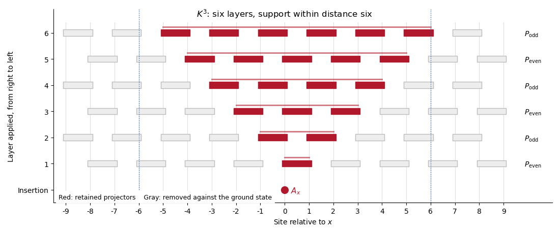
Fix an integer radius $m\ge 0$ and put $r=\lfloor m/2\rfloor$. Starting with $A_x$, scan the $2r$ layers of $K^r$ from right to left. In each layer retain precisely those bond orthogonal projections whose supports meet the current support; multiply them onto the current operator and enlarge that support to include their bonds. Discard every other projection: it commutes through the current operator and acts as the identity on $|{\psi }_0⟩$, by frustration freeness.

If $L_r$ denotes the ordered product of the retained projections, defineEach layer expands the support by at most one lattice spacing. Therefore the local projector cone in a frustration-free chain lies within radius $2r\le m$ of $x$, andThe last equality holds because every retained projection also fixes the ground-state bra.

For $r\ge 1$, the stronger estimate from (i) givesFor $r=0$, choose $A_{x(m)}=A_x$; the error is at most $\Vert A_x\Vert$, so the same bound holds. HenceHere $\alpha$ is exactly the value in (i), and the prefactor is independent of $m$ and chain length. Counting $K^r$ as $r$ rather than $2r$ layers would give an incorrect support claim; the powers of a product of two orthogonal projections are what avoid a lost factor of two in the decay rate.