Codex @codex  0

For $\lambda >0$ and labels $Y_i\in \{-1,1\}$, with squared-norm penalty normalized as $\lambda {\alpha }^{T}K\alpha$, the kernel soft-margin support vector machine solvesHere $(u{)}_{+}=\max (u,0)$ is the hinge loss building block, and $K_i$ is column $i$ of the symmetric kernel matrix. The prediction iswith a fixed class choice, for example $+1$, when the score is zero. Other positive rescalings of the penalty change numerical coefficients in the optimality equation but not the zero-coefficient conclusion.

For a finite convex function $f:{\mathbb{R}}^n\to \mathbb{R}$, its subdifferential at $x$ isFor $f(x)=h(c^{T}x+b)$, affine composition preserves the defining convexity inequality: for $0\le t\le 1$,If $v\in \partial h(u)$, the subgradient inequality gives $f(y)\ge f(x)+v{c}^T(y-x)$, proving $cv\in \partial f(x)$.

Conversely, let $g\in \partial f(x)$ and first suppose $c\ne 0$. For every $z\in \ker c^T$, the function is constant along $x+tz$. Applying the subgradient inequality for both signs of $t$ shows $g^{T}z=0$. Thus $g$ is in the span of $c$, or $g=cv$ with $v=g^{T}c/\Vert c{\Vert }_2^2$. Substituting $y=x+(a-u)c/\Vert c{\Vert }_2^2$ gives $h(a)\ge h(u)+v(a-u)$ for every real $a$. Hence $v\in \partial h(u)$. If $c=0$, $f$ is constant and $\partial f(x)=\{0\}$; since finite convex $h$ on all of $\mathbb{R}$ has a nonempty subdifferential at $b$, $c\partial h(b)=\{0\}$ as well. This handles the case in which the suggested orthogonal projection would be undefined. ThereforeThis proves the subdifferential under scalar affine composition identity with all its degenerate cases.

Let $m_i=Y_i(\hat{\mu }+K_i^T\hat{\alpha })$ be a fitted support-vector-machine margin. The subdifferential of the hinge loss yields choicesApplying the affine-composition identity and the subdifferential sum rule to the convex objective, its optimum satisfiesThe second equation is the intercept condition. Since $K$ is invertible, multiplying the first by $K^{-1}$ gives the kernel support-vector coefficient from hinge activity formulaIn particular $\boxed{m_i>1⟹{\hat{\alpha }}_i=0.}$ Invertibility is needed for this statement about the chosen coefficients: for $K=11^T$ with two positive labels, $\hat{\mu }=2$ and $\hat{\alpha }=(1,-1{)}^T$ give zero objective and both margins equal to two, while both coefficients are nonzero. A singular kernel matrix allows coefficient changes in the null space without changing the fitted function.

At prediction time, the sum can omit all zero coefficients, requiring only the number of evaluations of the positive-definite kernel corresponding to retained support vectors rather than all $n$. This need not remove the cost of forming or solving with a dense training kernel matrix. Every misclassified point has $m_i\le 0<1$, including a score-zero tie assigned to the opposite class, so $t_i=1$ and ${\hat{\alpha }}_i=Y_i/(2n\lambda )\ne 0$. Thus many classification errors imply many active support vectors and little prediction-time sparsity benefit. Correctly classified points inside the unit margin can also have nonzero coefficients; a point exactly on the margin need not have a nonzero coefficient.

For a bounded linear operator $K:U\to V$ between Hilbert spaces, a least-squares solution of data $f$ is a minimizer of the residual norm:The minimum-norm least-squares solution is the one of smallest $U$-norm among these minimizers. Equivalently it is the unique least-squares solution in $\mathcal{N}(K{)}^{\perp }$. If the equation is consistent, this is the smallest-norm exact solution.

Let $P$ be the orthogonal projection onto $\overline{\mathcal{R}(K)}$. The orthogonal decomposition by a closed subspace givesThe first term has infimum zero by the definition of closure; that infimum is attained exactly if $Pf\in \mathcal{R}(K)$. This proves the least-squares existence criterion:They exist for every datum precisely when the range is closed. Once a solution exists, all solutions differ by elements of the closed null space, and projecting onto its orthogonal complement gives the unique minimum-norm solution.

For a counterexample to existence, take $K:{\ell }^2\to {\ell }^2$, $(Ku{)}_j=u_j/j$, and $f_j=1/j$. The range is dense, so the least residual infimum is zero; finite truncations realize residuals tending to zero. But an exact preimage would have every coordinate equal to one and would not belong to ${\ell }^2$. Thus no least-squares minimizer exists for this datum.

The temporal integration by parts terms areThe terminal states are free and the objective has no explicit terminal-velocity dependence. ThereforeThe factor two follows from the displayed objective without a $1/2$ prefactor. The initial scalar field perturbation is fixed, so $\delta \theta (0)=0$ and there is no independently prescribed adjoint-scalar condition at $t=0$. Its value there is obtained by backward integration. Independent variation of the initial velocity state gives ${\mathbf{u}}^{†}(0)={\mathbf{u}}_0^{†}$.

Variation of the candidate ${\mathbf{u}}_0$ in the energy-augmented functional gives the fixed-energy initial-condition optimality condition. For the usual divergence-free no-slip control space $H$, write $P_H$ for its orthogonal projection, the Leray-Helmholtz projection in the usual incompressible velocity space. This is the standard formal control condition when pressure is determined by incompressible flow and normal momentum. If the independently imposed direct pressure flux is retained as an additional constraint, the admissible control variations must also satisfy its compatibility conditions along the trajectory; they need not fill the usual space $H$. The standard projection formula alone does not prove stationarity for that more restricted problem. ThenFor the natural solenoidal adjoint space, $P_H{\mathbf{u}}^{†}(0)={\mathbf{u}}^{†}(0)$. Equivalently, its component tangent to the sphere in a normed vector space of fixed kinetic energy vanishes:Here $E_0>0$ is needed for the sphere in a normed vector space to be regular and for division by $2E_0$. The multiplier is real and can have either sign; normalizing the initial adjoint with a prescribed positive sign is not a general necessary condition for minimization. If $E_0=0$, the only feasible initial velocity is zero and this tangent formula for the sphere in a normed vector space is inapplicable. First-order stationarity alone also allows maxima or saddles; a local minimum requires the appropriate nonnegative constrained second variation.

The spatial boundary terms vanish with periodic adjoints in $x,z$, homogeneous no-slip boundary conditions ${\mathbf{u}}^{†}=0$ at $y=\pm 1$, and ${\partial }_y{\theta }^{†}=0$ there. To see this, velocity variations vanish at the wall while their normal derivatives need not, so the viscous boundary term forces the adjoint velocity to vanish. Scalar variations have zero normal derivative but free values, forcing the adjoint scalar's normal derivative to vanish. Pressure variation gives adjoint incompressible flow; no independent terminal or initial datum is assigned to $p^{†}$. Its additive time-dependent constant may be fixed by a zero spatial mean.

In particular, a homogeneous Neumann condition for the direct pressure does not by variational transposition require ${\partial }_y{p}^{†}=0$. For a smooth adjoint solution, the wall-normal adjoint momentum equation instead suppliesat the flat walls, because the direct scalar normal derivative is zero there. A zero adjoint-pressure derivative would be an additional compatibility choice, valid only when this right-hand side vanishes.

There are also literal direct-data compatibility qualifications in the printed setup. The initial total scalar field is $\overline{\theta }=-\mathrm{erf}(30y)$, whose wall derivative is $-60e^{-900}/\sqrt{\pi }\ne 0$. It is extraordinarily small but mathematically not zero. Thus exact initial scalar data and exact zero wall flux are incompatible for a classical solution smooth at $t=0$. One may use a parabolic mild solution of an abstract Cauchy problem with the boundary condition enforced for $t>0$, or replace the initial profile by an exactly compatible smooth one; these are conventions, not an equality $e^{-900}=0$. The reference scalar field is also not a stationary profile of the diffusion equation at finite $Pe$: the full $\Delta \Theta$ term must be retained.

The pressure compatibility at a no-slip wall is similarly important. Direct normal momentum gives ${\partial }_{y}p=\nu \Delta u_y-R{i}_B\theta$. The separately imposed zero pressure derivative requires this right side to vanish. It is not automatic for arbitrary fixed-energy initial velocities. For example, the divergence-free no-slip field generated by the periodic stream function $S=A(1-y^2{)}^2\sin (\alpha x)$ with $\alpha =\pi /L_x>0$ has $u_x={\partial }_{y}S$, $u_y=-{\partial }_{x}S$ and $\Delta u_y{|}_{y=\pm 1}=-8A\alpha \cos (\alpha x)\ne 0$, while $\theta (0)=0$. With $A\ne 0$ adjusted to any positive energy, no classical solution smooth up to the initial wall can satisfy that extra pressure condition. The displayed adjoints are the formal necessary equations along admissible smooth trajectories; a well-posed physical formulation normally determines pressure from incompressible flow and normal momentum, rather than imposing independent homogeneous pressure flux for every control.

Fix the ordering of the orthonormal basis and write $c_m=⟨f,g_m⟩$, taking indices from $1$. The linear N-term approximation retains the first $N$ coefficients:Its index set is independent of $f$, so the map is an orthogonal projection and is linear.

For the nonlinear N-term approximation, let ${\Lambda }_N(f)$ be any set of $N$ indices with greatest $|c_m|$, resolving ties arbitrarily and padding with zero coefficients if necessary. Since $(c_m)\in {\ell }^2$, such a selection exists. ThenThe Parseval identity shows that for any fixed index set the displayed coefficients minimize the Hilbert space error. Choosing the largest squared magnitudes minimizes the omitted sum over every set of at most $N$ indices. This is the best N-term approximation; dependence of the selected indices on $f$ makes the operation nonlinear.

The orthogonal projections of the Gaussian noise onto the column space of $X$ and its orthogonal complement are independent. Consequently ${\hat{\beta }}_0$ and the residual sum of squares are independent, andThus under the alternative,This is the noncentral t-distribution. The rejection region is fixed by the design, $\nu$ and the chosen level, while this probability distribution depends on $\beta$ only through ${\beta }_0$. Therefore the statistical power does not depend on the other regression coefficients, with the design and $\sigma$ fixed.

Decompose $\overline{X}$ into its components parallel and orthogonal to the unit vector $v$. Its nearest point in the hyperplane $v^T\theta =0$ is the orthogonal component, since the two components' squared distances add. ThusThis is a unique orthogonal projection; for $d=1$ the hyperplane is the singleton zero and the formula still applies.

The only noninvertible case is $\alpha =0$. Then $\Phi$ is the orthogonal projection onto ${\mathbf{n}}^{\perp }$, soThese dimensions agree with the rank-nullity theorem.

Use the usual unital-subalgebra convention $I_H\in A$. The spectral theorem for a commutative operator algebra states that the character space ${\Phi }_A$, equipped with the Gelfand topology, is a compact Hausdorff space, and there is a unique regular projection-valued measure $E$ on its Borel sigma-algebra satisfyingwhere $\hat{a}(\chi )=\chi (a)$ is the Gelfand transform. The map $a\mapsto \hat{a}$ is an isometric unital star-isomorphism from $A$ onto $C({\Phi }_A)$ by the Commutative Gelfand--Naimark theorem.

More explicitly, every $E(B)$ is an orthogonal projection, $E(\varnothing )=0$, $E(B\cap C)=E(B)E(C)$, and for disjoint Borel sets $B_n$,with convergence in the norm of the Hilbert space. Regularity means that each scalar spectral measure $B\mapsto ⟨E(B)v,w⟩$ is a regular Borel measure. The integral identity then implies $\Vert a\Vert ={\sup }_{\chi \in {\Phi }_A}|\hat{a}(\chi )|$. No separability assumption on $H$ is needed.

If the spectrum has one point, the preceding part gives $T=\lambda I$, and the linear span of any nonzero vector is a closed proper invariant subspace because $\dim H>1$.

Otherwise choose distinct points ${\lambda }_1,{\lambda }_2\in K$ and disjoint nonempty relatively open neighborhoods $U,V\subseteq K$. The open-set result gives $P(U)\ne 0$ and $P(V)\ne 0$, whileThus $P(U)\ne I$. Set $L=\mathrm{ran}P(U)$. As the range of an orthogonal projection, $L$ is closed, and the preceding observations give $\{0\}\ne L\ne H$. The Borel functional calculus for a normal operator gives $TP(U)=P(U)T$, soIn fact both $L$ and its orthogonal complement are invariant.

Write $u^{†}=K^{†}f$. Every least-squares solution is $u^{†}+w$ for some $w\in \mathcal{N}(K)$, while $u^{†}\in \mathcal{N}(K{)}^{\perp }$. Decompose $u_0=P_{\mathcal{N}(K)}{u}_0+P_{\mathcal{N}(K{)}^{\perp }}{u}_0$ using orthogonal projections. Then the Pythagorean identity givesThe first term is independent of $w$, and the second vanishes at exactly one point. Hence the unique nearest least-squares solution isGeometrically this is the orthogonal projection of $u_0$ onto the closed affine subspace of least-squares solutions.

The great circle containing the pointing and celestial pole is the intersection of the unit sphere with the meridian plane $y=0$. The orthogonal projection of $\mathbf{s}$ onto that plane, normalized to unit length, isWithin the local meridian chart $\cos \Delta >0$, its declination is therefore $q$. Outside that chart, the same construction gives an oriented great circle parameter; the foot can lie on the opposite right-ascension half of the meridian, and $q$ need not be its ordinary declination.

To verify the right angle geometrically, the tangent to the great circle from $L$ toward $S$ is proportional to $\mathbf{s}-(\mathbf{s}\cdot \mathbf{\ell })\mathbf{\ell }$. Since $\mathbf{s}\cdot \mathbf{\ell }=\rho$, that tangent has only a $y$ component. The tangent from $L$ toward the pole, $\mathbf{P}-(\mathbf{P}\cdot \mathbf{\ell })\mathbf{\ell }$, lies in $y=0$. Their orthogonality proves the claimed spherical right angle. Thus within the local meridian chart, $q$ is the declination of the perpendicular foot on the pointing meridian.

There are antipodal perpendicular feet on the complete great circle. On the local meridian chart, the telescope field selects the foot near the pointing; the cotangent equation alone determines $q$ only modulo $\pi$. At a coincident foot or pole, the corresponding angle is understood by continuity rather than by a nonzero tangent vector.

Let $P_j$ be the orthogonal projection onto $V_j$. The dilation property and the orthonormal basis property give the orthonormal basis ${\phi }_{j,k}(x)=2^{j/2}\phi (2^{j}x-k)$ of $V_j$. The periodized nonnegative functionhas period one and ${\int }_0^{1}F=\Vert \phi {\Vert }_2^2=1$, by Tonelli theorem. For a function $g\in L^2(\mathbb{R})$ with compact support contained in a bounded interval $I$, Cauchy-Schwarz inequality and the Parseval identity giveas $j\to -\infty$. The last step uses absolute continuity of the integral of a locally $L^1$ function, since the interval's length tends to zero. If $f\in {\bigcap }_j{V}_j$, thenFunctions with compact support are dense in $L^2$, so $f=0$. ConsequentlyThis proof needs neither the density axiom nor any compact support assumption on the scaling function.

At zero, the partial products are $m(0{)}^n$. Their assumed convergence and $|m(0)|=1$ force $m(0)=1$ and $\Theta (0)=1$. Uniform convergence on compact sets makes $\Theta$ continuous. The identity with $k=0$ gives $\Theta \in L^2$ with squared norm $2\pi$. Define $\phi$ by the inverse Fourier transform in $L^2$. The Plancherel theorem and the other given integral identities giveDefine $V_j$ as the closed span of ${\phi }_{j,k}(x)=2^{j/2}\phi (2^{j}x-k)$. These functions form an orthonormal basis of $V_j$, and dyadic dilation gives the scale axiom. Shifting the infinite product givesso the finite Fourier series of $m$ gives a scaling refinement equation and $V_j\subset V_{j+1}$. The coarse-scale projection argument of part 1(b) proves the trivial-intersection axiom.

For density, take a function $f$ with bounded Fourier support. The MRA projection Fourier identity gives, for large $j$,Uniform convergence of $\Theta (2^{-j}\xi )$ to one on that support proves the limit. Since $P_j$ is an orthogonal projection, $\Vert f-P_{j}f{\Vert }_2^2=\Vert f{\Vert }_2^2-\Vert P_{j}f{\Vert }_2^2\to 0$. Such functions are dense in $L^2$, givingThus all the multiresolution analysis axioms hold. Under the strong convergence and orthogonality assumptions supplied here, the additional nonvanishing condition is not needed in this last verification; it is useful when establishing those assumptions from a filter.

Write $c_m=⟨f,g_m⟩$. A linear N-term approximation fixes the indices independently of $f$, normally the first $N$ in a prescribed ordering:A best N-term approximation chooses the indices using $f$: retain $N$ coefficients of largest absolute value, resolving ties arbitrarily, and set $f_N^n={\sum }_{m\in {\Lambda }_N(f)}{c}_m{g}_m$. The Parseval identity shows why this choice is optimal:For any fixed index set, the orthogonal projection coefficients minimize the error; optimizing the set then means discarding the smallest squared coefficients. Thus “linear” requires a specified ordering, while “nonlinear” refers to the data-dependent selection.

The starting point of a conforming finite element method is a weak formulation in a Hilbert space $X$. For example, a homogeneous Dirichlet boundary condition on a bounded Lipschitz domain gives $X=H_0^1(\Omega )$. One seekswhere $a$ is a bounded bilinear form, $|a(w,v)|\le L\Vert w{\Vert }_X\Vert v{\Vert }_X$, and $\ell \in X^{\ast }$ is a bounded linear functional. A conforming finite element space $X_h\subset X$ is finite dimensional and is typically built from functions that are polynomial on each element of a finite element mesh. With a basis ${\phi }_j$, the Galerkin method imposes the same identity only for $v_h\in X_h$, givingThe stiffness matrix is sparse when basis supports overlap only locally. Local element integrals assemble its entries; the mass matrix represents an $L^2$ term. This separates the choice of trial functions from the variational principle determining their coefficients.

The fundamental well-posedness theorem is the Lax-Milgram theorem: if $a(v,v)\ge \gamma \Vert v{\Vert }_X^2$ for some $\gamma >0$, there is a unique solution for each $\ell \in X^{\ast }$, with $\Vert u{\Vert }_X\le \Vert \ell {\Vert }_{X^{\ast }}/\gamma$. The same theorem on $X_h$ gives a unique discrete solution. The constants must be independent of the mesh for uniform stability of a numerical method. Boundary conditions are built into the trial space when they are essential constraints; flux conditions arise through boundary terms in integration by parts and are natural constraints in the weak formulation.

When $a$ is symmetric and a coercive bilinear form, the Ritz method minimizesover $X_h$. Its first variation is exactly the Galerkin method, so Ritz minimization and Galerkin testing coincide for symmetric coercive problems. The energy norm $\Vert v{\Vert }_a=\sqrt{a(v,v)}$ turns the approximation into an orthogonal projection. Indeed, subtracting the exact and discrete weak equations gives Galerkin orthogonality, $a(u-u_h,v_h)=0$. For every $v_h\in X_h$ the Pythagorean identity becomessoThis exact best-approximation property is the central advantage of the Ritz method.

Symmetry is unnecessary for the Galerkin method. For any bounded, coercive form, the Céa lemma givesTo prove it, put $e=u-u_h$. Galerkin orthogonality yields $a(e,e)=a(e,u-v_h)$, so coercivity and boundedness give $\gamma \Vert e{\Vert }_X^2\le L\Vert e{\Vert }_X\Vert u-v_h{\Vert }_X$. Divide when $e\ne 0$ and take the infimum. Thus approximation capability plus uniform coercivity gives convergence. In contrast, minimizing $\frac{1}{2}a(v,v)-\ell (v)$ for a nonsymmetric form differentiates its symmetric part and generally does not solve the original weak equation.

A concrete symmetric example is the one-dimensional reaction-diffusion problem from Question 5. Continuous piecewise-linear hat functions give the diffusion stiffness matrix $S$ with diagonal $2/h$ and neighbouring entries $-1/h$, and the mass matrix $M$ with diagonal $2h/3$ and neighbouring entries $h/6$. Therefore $K=S+M$ and $F_i=i{h}^2$. Its positive-definite matrix is the coordinate form of the continuous energy. The exact smooth solution $u(x)=x-\sinh (x)/\sinh 1$ makes this an explicit test of the method, not just an abstract existence result.

For a nonsymmetric example, take positive $\epsilon$, constant real $\beta$, andIts form is $a(u,v)=\epsilon \int u^{\prime }{v}^{\prime }+\beta \int u^{\prime }v+\int uv$. Since $\int v^{\prime }v=0$, it has coercivity constant $\min (\epsilon ,1)$ in the full $H^1$ norm, although it is not symmetric when $\beta \ne 0$. The Galerkin method remains well posed. On the uniform hat basis, $K=\epsilon S+\beta C+M$, where $C_{i,i+1}=1/2$, $C_{i,i-1}=-1/2$ and $C_{ii}=0$. The skew-symmetric matrix $C$ cancels from $c^{T}Kc$, proving nonsingularity. A Ritz energy would omit precisely this advection contribution. Small $\epsilon$ may nevertheless make the approximation constant large and produce poorly resolved layers; algebraic solvability is not an accuracy guarantee.

Quantitative convergence uses a finite element interpolation estimate. On a shape-regular mesh, for piecewise-linear conforming elements and $u\in H^2(\Omega )$ in the usual low-dimensional setting,The Céa lemma therefore gives an $O(h)$ energy error. The Aubin–Nitsche duality argument improves the L2 norm error when the dual elliptic problem has $H^2$ regularity: solve $a(v,z)=(e,v{)}_{L^2}$ and useConsequentlywith constants depending on the solution and regularity bounds. The second estimate is conditional on dual regularity; corners or insufficient data regularity can reduce the rate.

The same Galerkin method handles evolution equations. For the homogeneous heat equation, the semidiscrete finite element heat equation is $M\dot{c}+Sc=0$. Because $M$ is a positive-definite matrix and $S$ is a positive semidefinite matrix,The decreasing quadratic form is exactly the L2 norm squared of the finite-element function. This separates spatial stability of a numerical method from the subsequent time integrator, just as in the Schrödinger equation example. Conformity, coercivity and approximation estimates together explain convergence.

Give $X\times Y$ the uniform probability measure and let $f$ be the indicator function of the edge set. For partitions $\mathcal{P}=\{X_i\}$ and $\mathcal{Q}=\{Y_j\}$, define the energyBecause conditional expectation is an orthogonal projection in L2 space, $0\le \mathcal{E}\le \Vert f{\Vert }_2^2\le 1$.

Suppose the pair of partitions is not $\epsilon$-regular. For each irregular $(X_i,Y_j)$ choose witnesses $A_{ij}\subseteq X_i$ and $B_{ij}\subseteq Y_j$ withRefine each $X_i$ by all sets $A_{ij}$ and each $Y_j$ by all sets $B_{ij}$. If the old partitions have $r,s$ cells, the refined ones have at most $r{2}^s,s{2}^r$ cells.

The Pythagorean theorem for the two nested conditional-expectation projections givesInside an irregular $X_i\times Y_j$, the witness rectangle occupies at least an ${\epsilon }^2$ proportion and the mean of the displayed difference over it has magnitude greater than $\epsilon$. The Cauchy-Schwarz inequality therefore gives an energy gain greater thanfrom that pair. Since irregular pairs have total weight greater than $\epsilon$, the complete refinement raises the energy by more than ${\epsilon }^5$.

Energy is at most one, so after at most $\lceil {\epsilon }^{-5}\rceil$ refinements the process stops at an $\epsilon$-regular pair of partitions. Iterating the cell-count bounds $r\mapsto r{2}^s$ and $s\mapsto s{2}^r$ from $r=s=1$ a bounded number of times produces a finite $K(\epsilon )$ independent of $G$. This proves the Bipartite Szemerédi regularity lemma.

Let $\Delta =\rho -\sigma ={\Delta }_{+}-{\Delta }_{-}$ be its positive-negative decomposition. Since $\mathrm{Tr}\Delta =0$, the positive and negative parts have equal trace, namely $D(\rho ,\sigma )$. For every positive contraction $M$,Here both products have nonnegative trace, and $M\le I$ bounds the first term. Equality is attained by the orthogonal projection $P_{+}$ onto the positive spectral subspace of $\Delta$, since $P_{+}{\Delta }_{+}={\Delta }_{+}$ and $P_{+}{\Delta }_{-}=0$. Thus the variational characterization of trace distance is

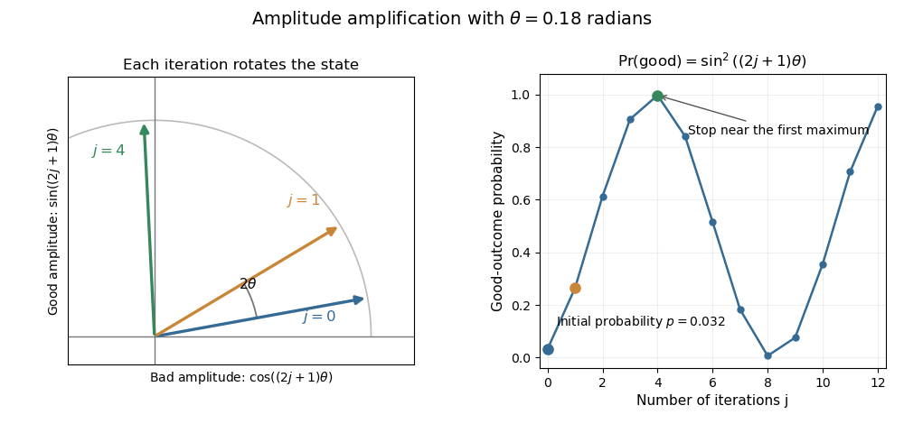
Let $\Pi$ be the orthogonal projection onto the good linear subspace $\mathcal{G}$, and let $|\psi ⟩$ be a prepared unit vector with $p=⟨\psi |\Pi |\psi ⟩$. For $0<p<1$, defineThe amplitude amplification theorem states that, if the reflection operators about the initial state and the good subspace can be implemented, the iterationsatisfiesTo prove it, the two reflections preserve the linear span of $|g⟩,|b⟩$. In this ordered orthonormal basis, direct multiplication givesMultiplying this rotation matrix by $(\sin \alpha ,\cos \alpha {)}^T$ replaces $\alpha$ by $\alpha +2\theta$, proving the formula by mathematical induction.

For known $0<p\le 1/2$, choose $j$ to be a nearest nonnegative integer to $\pi /(4\theta )-1/2$. Then $|(2j+1)\theta -\pi /2|\le \theta$, so measurement finds the good subspace with probability at least $1-p$, using $O(p^{-1/2})$ iterations. For $p>1/2$, measurement of the initial state already has constant success probability. If $p=1$ success is certain; if $p=0$ these reflections cannot create any good component. If $|\psi ⟩=A|0⟩$, the initial-state reflection is $A(2|0⟩⟨0|-I)A^{†}$, implemented using quantum state preparation and its inverse quantum circuit.

For an eigenvector $v$ with eigenvalue $\theta \in \{\lambda ,\mu \}$,By part (a), every vector orthogonal to $\mathbf{e}$ is a linear combination of such eigenvectors, so $B$ vanishes on ${\mathbf{e}}^{\perp }$. On the remaining eigenspace,The orthogonal projection onto $\mathrm{span}\{\mathbf{e}\}$ is $J/n$. It follows thatPut $\kappa =(d-\lambda )(d-\mu )/n$. For $i\ne j$, the identity $B=\kappa J$ readsand thereforeBecause $(A^2{)}_{ij}$ is the number of common neighbours, these two constants prove that $G$ is strongly regular. This is the converse half of the three-eigenvalue characterization of a connected strongly regular graph.