Past exam of the mathematics course of the University of Cambridge / 2001 / iii / Paper 44 (Slow Viscous Flow)

Put $r=|\mathbf{x}|$. In the Unscaled Papkovich–Neuber representation, choose the componentwise harmonic vector fieldBoth $\mathbf{\Omega }\times \mathbf{x}$ and $(\mathbf{\Omega }\times \mathbf{x})/r^3$ are harmonic away from the origin: the latter is a linear combination of derivatives of the harmonic function $1/r$. Also $\mathbf{x}\cdot \mathbf{\Phi }=0$, so the representation gives $\mathbf{u}=f(r)\mathbf{\Omega }\times \mathbf{x}$. The no-slip boundary condition requires $f(a)=1$ and $f(b)=0$, givingThus the Rotational Stokes flow between concentric spheres isThe divergence of $\mathbf{\Phi }$ is zero: the cross-product field itself has zero divergence, and $\nabla f$ is radial and perpendicular to $\mathbf{\Omega }\times \mathbf{x}$. Hence $p=2\mu \nabla \cdot \mathbf{\Phi }=0$ in this pressure gauge.

There is also a symmetry argument. Take the rotation axis as the polar axis. Linearity of Stokes flow makes velocity and pressure perturbations change sign when the rotation reverses. Reflection in any plane containing that axis reverses the axial rotation vector. Combined with axial symmetry, this excludes meridional velocity components and forces the pressure perturbation to be both unchanged and sign-reversed by that reflection. Equivalently a purely azimuthal axisymmetric Stokes flow has no meridional component of its vector Laplacian, so its meridional pressure gradient vanishes. Thus the pressure is constant; setting that arbitrary constant to zero gives the same result without solving the radial coefficients.

For the Newtonian fluid stress tensor, let $\mathbf{q}=\mathbf{\Omega }\times \mathbf{x}$. The symmetric part of the velocity gradient isbecause the gradient of rigid rotation is antisymmetric. Consequently the full stress tensor, with $p=0$, isFor $\mathbf{\Omega }=\Omega {\mathbf{e}}_z$, its only nonzero spherical-coordinate components are ${\sigma }_{r\varphi }={\sigma }_{\varphi r}=-3\mu B\Omega \sin \vartheta /r^3$. On the inner sphere the traction exerted by the fluid, using the sphere's outward normal $\mathbf{n}$, isIts torque isusing $\int n_i{n}_{j}d\omega =4\pi {\delta }_{ij}/3$. Therefore the applied Torque in rotational Stokes flow between concentric spheres isFor $b\gg a$, the relevant speed and length are $\Omega a$ and $a$, so negligible inertia requires the rotational Reynolds numberFor a narrow gap $d=b-a\ll a$, the viscous gradients are controlled by $d$, not $a$. A centrifugal acceleration of scale ${\Omega }^{2}a$ is then compared with viscous scale $\mu \Omega a/d^2$, rather than $\mu \Omega /a$. Their ratio is $\rho |\Omega |d^2/\mu$. This explains why the large-gap condition is not a necessary narrow-gap criterion; a thin gap greatly strengthens viscous resistance. This base-flow scaling is distinct from a criterion for stability to arbitrary short-scale disturbances.

The Minimum-dissipation theorem for Stokes flow compares a Stokes solution with all sufficiently regular incompressible trial velocities in the same fluid domain that have the same prescribed boundary velocities. With no body-force work, the dissipation functional isIf $\mathbf{v}=\mathbf{u}+\mathbf{w}$ and $\mathbf{w}=0$ on the prescribed boundary, integration by parts with $\nabla \cdot \mathbf{\sigma }(\mathbf{u})=0$ and $\nabla \cdot \mathbf{w}=0$ makes the cross term vanish. ThusThe comparison fixes velocities, rather than applied torques or forces.

Now let the particles take their actual rigid translations and rotations in the particle-containing flow. Extend the fluid velocity through each particle by its rigid velocity. No-slip boundary conditions make this extension continuous; rigid motion has zero rate-of-strain tensor and zero divergence. The extension is therefore an admissible trial field in the original particle-free annulus, and its dissipation equals that of the fluid outside the particles. Hence $D\ge D_0$.

The Stokes boundary-work identity gives $D=\mathbf{G}\cdot \mathbf{\Omega }$. The outer sphere is stationary, the maintained inner sphere has zero translational velocity, and every added particle has zero total force and torque, so none of those other boundaries contributes power. Likewise $D_0={\mathbf{G}}_0\cdot \mathbf{\Omega }$. ThereforeFor nonzero rotation and a particle of positive volume the inequality is strict: equality in the dissipation identity would force the extension to be the unique original flow, but that original flow has nonzero strain on every open particle region, whereas a rigid interior has zero strain. This proves that force-free inclusions increase rotational resistance:No dilute-suspension approximation or assumption about the particle shapes was used.

In a slender symmetric viscous sheet, the two broad faces have zero tangential traction. A cross-thickness variation of $w$ on the thickness scale would produce leading shear $\mu w_x$, whereas $\mu u_z$ is smaller by the square of the aspect ratio. The leading transverse momentum balance and the shear-free conditions therefore give $w_x=0$: write $w=w(z,t)$.

Incompressibility gives $u_x=-w_z$. Symmetry about $x=0$ sets the integration constant to zero, soThe normal traction on either nearly vertical face matches the ambient hydrostatic pressure, giving ${\sigma }_{xx}=-p_a$ to leading order. The Newtonian fluid stress tensor then yieldsThe factor four is the planar extensional resistance, as in the planar viscous-sheet stretching equations, rather than the factor three for uniaxial extension with two contracting transverse directions.

The following slice diagram shows all axial-force contributions per unit $y$-width; the end arrows indicate positive tensile stress and reverse if that signed stress is negative.

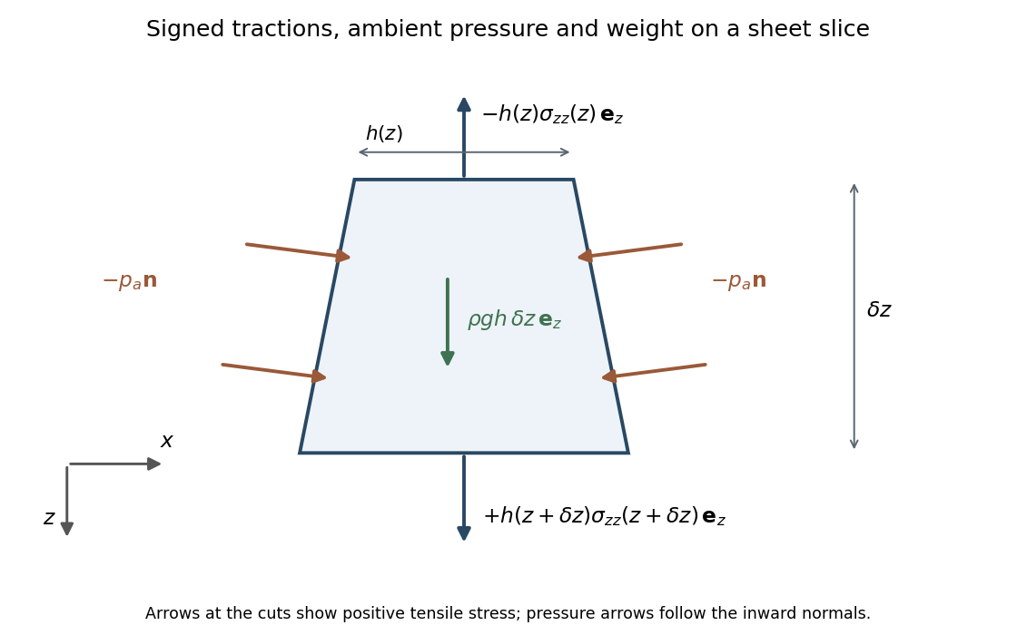
The two end tractions have net $z$-component ${\partial }_z(h{\sigma }_{zz})\delta z$. The normal pressure on the inclined side faces contributes $p_a{h}_z\delta z$, and gravitational acceleration gives the weight $\rho gh\delta z$. Hence force balance isSubstitute the stress expression and $p_a^{\prime }={\rho }_{a}g$:soKeeping the side-pressure component is essential: dropping it would retain an incorrect dependence on the arbitrary ambient pressure level. The remaining equation from conservation of mass isIt follows either by integrating incompressibility across the moving faces or directly from the face kinematic boundary condition.

When effective gravitational acceleration vanishes, $4\mu h{w}_z$ is independent of $z$. It equals the applied excess tensile force $F(t)$, with ambient pressure removed from the end loading. Along a material element labeled by its initial position $z_0$,Integration gives uniform material thinning under planar-sheet tension:A material interval conserves its area: $h(z,t)dz=h_0(z_0)d{z}_0$. ThusWith the specified fixed material origin, integrate the latter relation to obtainThese formulas hold while the material thickness remains positive.

For the quadratic initial profile, put $q=H-\Delta >0$. If $k\ne 0$, evaluating the integral at $z_0=L_0$ givesFor $k=0$ it instead givesFor a constant positive pulling force, $\Delta =Ft/(4\mu )$ first reaches the minimum initial thickness $H$ atBoth expressions for $L$ diverge there. Write $q=F(t^{\ast }-t)/(4\mu )$. If $k\ne 0$, the inverse tangent tends to $\pi /2$ and $\Delta \to H$, givingFor $k=0$,This is finite-time extension of a quadratically thickened sheet. With nonzero $k$, the dominant extension comes from the small material region $|z_0|=O(\sqrt{q/H}/|k|)$ near the thickness minimum, where the integrand is proportional to $1/(q+H{k}^2{z}_0^2)$. Its width shrinks like $\sqrt{q}$, giving an integrated divergence $q^{-1/2}$. The fixed ends are asymptotically far away in those local coordinates, so $A$ does not depend on $L_0$. For a uniform sheet the entire material interval has denominator $q$, giving the stronger $q^{-1}$ divergence and retaining its length in $A$. The singularity is a prediction of the ideal slender-sheet model as its minimum thickness tends to zero.

For a stationary film of uniform thickness, thermal conduction gives $T_{zz}=0$, so $T=T_0+cz$. The cooling boundary condition determines $c$:Consequently the surface temperature isThis is the quasistatic temperature of a conductively cooled film, with a weak-cooling expansion when $\alpha h/\kappa \ll 1$.

Let the thickness and longitudinal scales be $h_{\ast },L$, with $ϵ=h_{\ast }/L\ll 1$. Incompressibility gives transverse speed of order $ϵU$, and film evolution has the kinematic time scale $L/U$. For the temperature variation scale $\Theta$, longitudinal diffusion divided by transverse diffusion is $h_{\ast }^2/L^2={ϵ}^2$. Each advective term, and the time derivative on that evolution scale, divided by transverse diffusion isThus ${ϵ}^2\ll 1$ and $Pe\ll 1$ make the leading thermal profile locally linear and quasistatic. Retaining the weak-cooling condition gives the same surface-temperature approximation with the local $h(x,t)$. For any independently imposed faster time variation one would also require its thermal relaxation ratio $h_{\ast }^2/(\kappa t_{\mathrm{evol}})$ to be small.

Define the positive surface-tension gradient coefficientThe weak-cooling approximation gives ${\gamma }_s\simeq {\gamma }_0+Bh$, so the Marangoni stress is ${\gamma }_{s,x}=B{h}_x$. The Young–Laplace equation gives the leading liquid pressure $p=p_a-{\gamma }_0{h}_{xx}$, with constant ambient pressure. In lubrication theory, $p_z=0$ and $\mu u_{zz}=p_x$. The no-slip boundary condition at the wall and the tangential surface condition $\mu u_z(h)={\gamma }_{s,x}$ giveHence the volume flux isConservation of mass gives the thermocapillary thin-film equationThe replacement of surface tension by ${\gamma }_0$ in the capillary term needs $B{h}_{\ast }/{\gamma }_0\ll 1$. For comparable capillary and thermocapillary fluxes,so the fractional tension change is only $O({ϵ}^2)$. Both the tension correction to $\gamma h_{xxx}$ and the differentiated-tension contribution ${\gamma }_x{h}_{xx}$ are then higher-order. Weak cooling alone would not justify that replacement if $|{\gamma }^{\prime }|\Delta T/{\gamma }_0$ were allowed to grow without bound.

The capillary term smooths the film: a crest has negative curvature and higher liquid pressure, causing flow away from it. The thermal term has the opposite effect. A thicker region has a colder surface and therefore higher surface tension; Marangoni stress pulls surface fluid toward that region, reinforcing the thickness disturbance. These mechanisms give fourth-order damping and second-order growth respectively.

Use $H=h/\hat{h}$, $X=ϵx/\hat{h}$, and $\tau =t/\hat{t}$. The two dimensionless flux-divergence coefficients are $B{ϵ}^2\hat{t}/(2\mu )$ and ${\gamma }_0{ϵ}^4\hat{t}/(3\mu \hat{h})$. Setting both equal to one gives the balanced scales for a thermocapillary film:These choices yield $H_{\tau }+(H^2{H}_X{)}_X+(H^3{H}_{XXX}{)}_X=0$. The predicted $ϵ$ must be small for the assumed long-wave approximation.

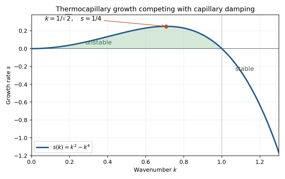
Linearize about $H=1$ using a normal mode of amplitude $\delta$. The resulting equation is $s-k^2+k^4=0$, so the dispersion relation isModes with $0<|k|<1$ grow, while $|k|>1$ modes decay. Differentiating $s$ gives the most unstable wavenumbersThe physical fastest wavenumber is $ϵ/(\sqrt{2}\hat{h})$.

For a positive steady film with zero volume flux, $H^2{H}_X+H^3{H}_{XXX}=0$. Divide by $H^3$ and integrate once:Choosing the thickness scale so that $H=1$ when $H_{XX}=0$ sets $C=0$. Multiply $H_{XX}=-\ln H$ by $H_X$ and integrate to obtain the zero-flux thermocapillary film profiles relationThus the stated potential is $V(H)=H(\ln H-1)$ and the integration constant $E$ is the corresponding first integral.

For a stationary solid skeleton, the Darcy velocity $\mathbf{u}$ is liquid volume transport per unit total cross-sectional area, while the pore velocity $\mathbf{v}$ is the intrinsic mean fluid velocity within the connected pore space. ThusFor an incompressible liquid in a saturated region, conservation of mass is ${\varphi }_t+\nabla \cdot \mathbf{u}=0$. With time-independent but spatially varying porosity, it becomesnot generally $\nabla \cdot \mathbf{v}=0$. Neglecting dispersion, a fluid interface is advected by the pore velocity; its mean normal speed is $V_n=\mathbf{v}\cdot \mathbf{n}=\mathbf{u}\cdot \mathbf{n}/\varphi$.

For the thin layer on the inclined plane, the gravitational acceleration components are $g\sin \theta$ downslope and $-g\cos \theta$ normal to the plane. The hydrostatic approximation and constant pressure $p_a$ above the current giveWith permeability of a porous medium $k(z)$, Darcy's law therefore givesHere $u_x,u_y$ denote the components of the Darcy velocity. Integrate over depth, using the prescribed power laws:Both integrals are finite for the positive exponents in the model. Conservation of the stored fluid gives ${\mathcal{V}}_t+{\nabla }_{x,y}\cdot \mathbf{Q}=0$, orFor $0<\theta <\pi /2$, set $X=x\tan \theta$, $Y=y\tan \theta$ andSince $\cos \theta {\tan }^2\theta =\sin \theta \tan \theta$, the depth-dependent inclined porous-current equation isThe longitudinal flux carries fluid downslope, while the thickness-gradient terms spread it. The degenerate horizontal or vertical slope limits need their own coordinate scaling.

Far downslope let the typical height be $H(X)$ and the cross-slope half-width be $W(X)$. Slenderness gives $W\ll X$ and slowly varying longitudinal thickness. In a steady porous gravity current, the longitudinal spreading term is smaller than advection by the ratio $H/X$, while longitudinal diffusion relative to transverse diffusion is of order $(W/X{)}^2$. Thus the leading balance isIntegrating across the finite current, with zero flux through its dry side edges, makes the leading downslope volume flux constant:Balancing the two differential terms givesEliminate $H\propto W^{-1/\beta }$ to find the far-downslope width of a constant-flux porous current:The typical height is correspondingly $H\propto X^{-1/(2\beta +1)}$. For every $\beta >0$, the width exponent is less than one half, so $W/X\to 0$ and $H/X\to 0$, consistent with the discarded longitudinal terms. The porosity exponent $\alpha$ drops out because it enters storage, which has zero time derivative in this steady problem.

For constant porosity and permeability, the equation is $h_T+h_X={\nabla }_{X,Y}\cdot (h{\nabla }_{X,Y}h)$. Under $\tau =T$, $\xi =X-T$, $\eta =Y$, the chain rule gives $h_T=h_{\tau }-h_{\xi }$ and $h_X=h_{\xi }$. Thus the moving-frame porous medium equation isIts conserved mass is $M=\iint hd\xi d\eta$.

There is a source inconsistency in the printed volume formula. Actual liquid volume is $V=P\iint hdxdy$. The stated coordinates have Jacobian determinantso the volume Jacobian for downslope stretched coordinates requiresThe printed factor ${\tan }^2\theta$ in the first expression is its reciprocal and cannot be proved with these coordinates. For example, at $\theta =\pi /6$ an integral equal to one corresponds to actual volume $3P$, whereas the printed formula gives $P/3$. The physical-volume normalization below uses the corrected Jacobian.

Let $r=\sqrt{{\xi }^2+{\eta }^2}$. For the source-type axisymmetric similarity solution, putMass conservation imposes $a=2b$, and balancing $h_{\tau }$ against $\nabla \cdot (h\nabla h)$ gives $a+1=2a+2b$. Hence $a=1/2$ and $b=1/4$. The profile equation isMultiplying by $s$, the left side is $-\frac{1}{4}(s^{2}f{)}^{\prime }$. Integration and regularity at the origin giveWhere $f>0$, divide by $sf$ to obtain $f^{\prime }=-s/4$, soSet the profile to zero beyond this front. The mass normalization isTherefore the two-dimensional Barenblatt profile for quadratic porous-medium diffusion iswhere $[q{]}_{+}=\max (q,0)$. Its radius and central thickness areThe profile is regular at the center, its flux $-h{h}_r$ vanishes at the dry edge, and the front speed $r_N^{\prime }=r_N/(4\tau )$ equals the limiting advective speed $-h_r$ there. Its support shrinks to the release point as $\tau \downarrow 0$ while its mass stays $M$, giving the concentrated initial release in the weak sense.

In physical coordinates its center travels atand $r=\tan \theta \sqrt{(x-x_c{)}^2+y^2}$ with $\tau =\rho gK\sin \theta \tan \theta t/(\mu P)$. If the printed volume expression were instead adopted merely as a definition of a formal parameter $\tilde{V}$, the same profile would use $M=\tilde{V}/(P{\tan }^2\theta )$; that parameter would equal $V{\tan }^4\theta$, not the actual released fluid volume.