Let be the complementary modulus of the complete elliptic integral of the first kind. With , write the integrand as . Its logarithmic endpoint asymptotic of the complete elliptic integral comes from ; an expansion at fixed alone misses the constant accompanying the logarithm.
Choose an intermediate cutoff . In the endpoint region, the integral isOutside this region, the leading integral isThe arbitrary cutoff cancels in this matched asymptotic expansion, leavingThese are the divergent logarithm and the finite constant, the requested first two terms. If terms are instead grouped by powers of the complementary modulus, the next refinement is ; its coefficients agree with the DLMF expansion.
There are two contributing regions: an endpoint of width near , and a very narrow peak near . Both must be retained in the asymptotic expansion.
For the peak, set and . At fixed , and , so the integrand times approaches . This is the Lorentzian contribution from shrinking regularization. Its total contribution isFor example, cut off this region at : its scaled endpoints tend to infinity, while the changes in the exponential and logarithm inside the peak are exponentially small. The matched tails outside it are also exponentially small compared with the endpoint terms below.
At the endpoint, put and . To algebraic orders in , the regularizing denominator term is negligible there, giving the Laplace endpoint expansion with a logarithmic denominatorThis integral represents the endpoint expansion only; it is cut off before the original peak when making the argument precise. Since , with the Euler--Mascheroni constant, the first two contributions to the original integral areThe endpoint correction refines to , using derivatives of the gamma function. An application of Watson's lemma confined to would omit the leading peak contribution .
The Briggs-Bers technique starts with a temporal Laplace transform and spatial Fourier transform of a localized disturbance. The temporal inversion contour must initially lie above every temporal singularity. Lower it while deforming the spatial contour away from the roots of the dispersion relation. A collision of spatial branches originating on opposite sides of that contour can create a spatial pinch point. A contributing pinch with gives absolute wave-packet instability: exponential growth at a fixed position. Growth that is transported away while a fixed position decays is convective wave-packet instability. Solving finds candidate double roots, but does not by itself establish a pinch.
Substitution of the normal mode givesFor real wavenumber , the temporal growth rate isA nonzero real cubic coefficient in this expression makes it unbounded above on one end of the real axis. Once that coefficient vanishes, a positive quadratic coefficient also makes it unbounded above. Hence the bounded temporal growth condition for cubic dispersion isThe maximum is then , attained at and, when , at all real . A finite upper bound is necessary for choosing the initial temporal inversion contour; arbitrarily fast high-wavenumber growth prevents the usual Briggs-Bers criterion from defining that causal inversion for generic localized data.
For , the stationary candidates satisfysoEach candidate must pass the spatial-branch pinch test before its imaginary frequency is used. In particular, under the finite-growth conditions the real-wavenumber evolution has multiplier modulus at most . For integrable transformed initial data this bounds its fixed-position amplitude by a constant times that exponential. Thus a further necessary condition isThe false complex saddle in dissipative cubic dispersion illustrates why the second formal candidate cannot override this bound. For , the neighborhood gives a fixed-position impulse response proportional to : the cubic term is smaller on its scale. It therefore supplies the usual growing pinch when . The purely dispersive cases have stationary-phase algebraic prefactors instead. If , only the quadratic stationary point remains; if both derivative coefficients vanish, the equation is local multiplication and its growth is directly .
Write . At first order the amplitude-phase perturbation is . Expanding the cubic term in the focusing nonlinear Schrodinger equation gives . The constant terms cancel because . Separating real and imaginary parts yieldsFor the Fourier normal modes, these equations give and . Their determinant vanishes exactly whenThe focusing nonlinear Schrodinger modulation dispersion is negative for . One of the two frequencies then has positive imaginary part and grows exponentially: the constant state has modulational instability. The growth rate is , maximized at with value . Modes beyond the unstable band have real frequencies. The zero-wavenumber phase mode is neutral, with possible linear phase drift from a uniform amplitude perturbation.
First take . Set in the tail integral. This puts it in the endpoint form needed for Watson's lemma:The binomial coefficients are , where is the rising factorial. Integrating each endpoint term givesAlso, scaling the complete positive-ray integral gives . HenceThe endpoint term is exponentially small on this positive ray but must be retained for continuation to other sectors.
For complex , use so . Put and . The complete steepest descent contours from the cubic saddle are the rays , whose integrals are . Deform the finite contour onto one of these rays followed by the endpoint contour. The cubic exponential integral Stokes sectors giveFor , take below , between and , between and , and above . The corresponding algebraic coefficients are . A negative-real provides a useful sign check: is real and positive, so its two lateral algebraic coefficients must be complex conjugates.
The subdominant algebraic term switches across the Stokes linesThere is negative real and the endpoint exponential is dominant. The intervening anti-Stokes lines are , where and the exponential changes from growth to decay. The naming convention here distinguishes switching from equal exponential magnitude.
To resolve the jump near , optimally truncate the endpoint series at with , where . Let denote that truncated endpoint contribution. The Borel remainder for a cubic exponential integral derived in solution, together with the Gaussian pole transition for a large gamma parameter in solution, givesThis estimate is on the transition scale after optimal truncation. The error-function smoothing of a Stokes multiplier has width . Before the line and the coefficient is ; after it and the coefficient is , agreeing with the sector expansions. On the line the leading coefficient is their average. The original is an entire function; only its asymptotic decomposition has these sector-dependent coefficients.
The factorial tail provides the connection with the supplied Borel summation formula. Near the first switching line choose with , so is near the positive real axis and . The endpoint contribution through terms isWriting in its formal remainder, with , givesThus the Borel remainder for a cubic exponential integral, using the contour just above the pole specified in the paper, isThe continuation is chosen from the sector below the switching line. The term fixes that continuation; an alternative lateral pole contour would shift it by the corresponding residue. This is why the contour prescription must accompany the divergent factorial series.
Choose near the least term, so with . On writing , the parameter is . For ,The supplied Gaussian pole transition for a large gamma parameter therefore gives . Substitution in solution gives the smoothing formula in solution once the amplitude identity in solution is used.
The origin of the error function can also be seen locally. Set in the Borel integral. ThenThe saddle has become a Gaussian integral meeting a simple pole. With the upper-pole contour, the leading integral is . Its value at is from the indentation. Differentiating with respect to gives , so integration from zero gives . This independently fixes the sign and the half-jump on the Stokes line.
The gamma reflection formula, , at gives . Consequently, with and ,Multiplication by therefore changes the algebraic coefficient by exactly the required amount, from to . This confirms both the magnitude and phase of the smoothed jump, rather than only its error-function shape.
The square-root reaction problem with nested boundary layers has a small positive plateau , an left-end layer, and two distinct scales on the right. The broad right layer has width ; its inner edge needs a thinner transition to the plateau. A single right-end scale cannot describe both matches.
Here is a uniformly matched leading solution. Let solveusing the increasing branch below . DefineThen . For the right-hand branch, define by ; it tends to as . These formulas follow from the first integral of a square-root reaction layer and are expanded in solution and solution.
For sufficiently small , let . Then , so the right profile meets the prescribed order-one endpoint. The composite asymptotic expansion isThe subtraction removes the common plateau counted twice. Its boundary residuals are exponentially small: the right profile has almost reached at , and the left profile has almost reached at . In each active layer the opposite profile is exponentially close to its plateau, so the composite reproduces that layer's governing equation and the shared outer solution to the retained order.
The right transition location satisfies . Outside its thin transition, the broad right layer iswhere the bracket is positive; it matches through the thin layer to , rather than continuing as a fourth power on the wrong side. The dominant balances and the end-region matches are detailed below.
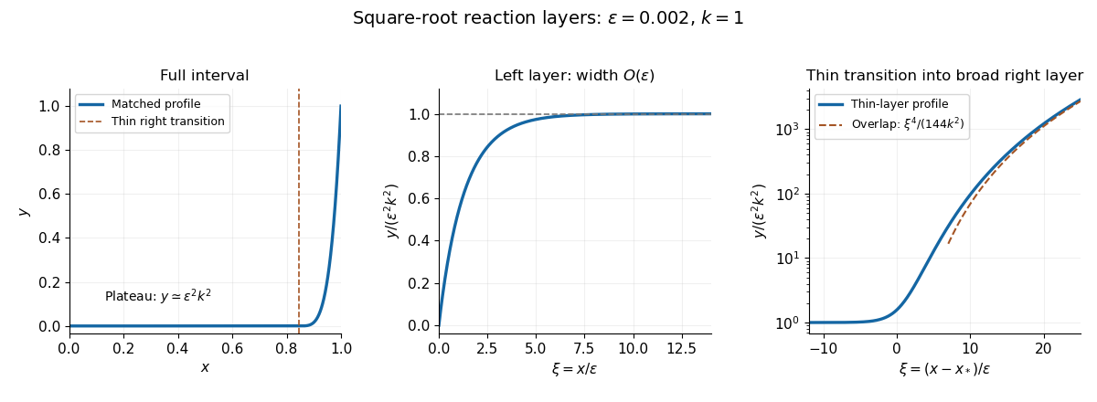
The left layer, small plateau and two right-hand scales of the square-root reaction problem
. Details. 
In the outer solution, derivative terms are small and , so . To resolve its mismatch with the zero left boundary, set , . The original equation becomes exactly . The left inner variable is therefore , with and as .
Multiplying by gives the first integral of a square-root reaction layer. Matching , fixes its constant:The positive derivative branch below begins with and approaches the plateau exponentially. Thus the left layer has thickness , not despite the coefficient on the original second derivative. Its small amplitude is essential in the dominant balance.
Put . The separated first integral of a square-root reaction layer gives a primitive as defined in solution. One can verify it directly: above the plateau,while below it the derivative has the opposite sign. Accordingly the increasing left profile uses , and the increasing right profile uses after choosing its translation constant.
As , the logarithm dominates:Hence the left profile approaches from below with , while the right profile approaches from above with as . These are precisely the required two plateau matching conditions. The absolute value in the logarithm is necessary to use the same real primitive on both sides.
For , the first integral of a square-root reaction layer reduces to . Integrating gives after a possible translation, orFor the right profile this large-positive- limit matches a broader scale with . Since and , the overlap isThus the translated layer lies between the outer plateau and the boundary layer. The large- primitive also gives , establishing the leading location .
For the broad right layer take and , so inside the interval. Its leading equation is , with . One integration gives . The positive derivative branch produces the integral parametrization in the hint.
Matching to a small, nearly flat plateau requires and at the inner edge, so the leading integration constant is . A positive order-one would leave a nonzero slope as ; a negative one would prevent that limit. For , integration with givesIts zero is at , namely . Near that edge it has the fourth-power overlap obtained in solution. The neglected reaction term becomes comparable to when , precisely where the thinner transition must restore it. The sketch in solution shows the plateau and both right-hand regions; extending the quartic profile past its inner edge would fail to match the positive plateau.
Use the method of multiple scales, , and write , . At first order,Removing the fundamental secular terms gives the averaged amplitude for position-dependent damping:where the brackets mean a full-period average. The initial conditions set and at leading order. For quadratic damping, and , givingThus the Van der Pol amplitude evolution yieldsThe leading amplitude approaches the stable value two. The small initial-velocity discrepancy introduced by the slow amplitude derivative is removed by the first-order correction and does not affect this leading approximation.
For , the period average vanishes: a half-period shift reverses the first factor and leaves the second unchanged. This is the zero first-order amplitude drift for odd damping. The averaged amplitude for position-dependent damping therefore has , while its first-order phase equation again has . With the initial conditions,The first-order forcing has no fundamental resonant component, so it produces bounded corrections rather than a secular amplitude change on this time scale. This statement concerns the leading approximation on .
For and positive amplitude , the averaged amplitude for position-dependent damping givesThe average is . Thus the absolute-value damping amplitude law isand as in the other cases. Consequently,The dissipation makes the leading envelope decrease algebraically in slow time. The absolute value is Lipschitz continuous, so the first-order averaging argument remains valid despite its corner at zero.
First assume the usual diffusion regime , with real; the complex-diffusion extension is described below. Substitution of a global normal mode givesSet to remove the first derivative, then put . The resulting oscillator equation isWriting gives the Hermite differential equation, . For a power series , its recurrence isTermination at degree requires . If it does not terminate in the appropriate parity, the series has a growing Gaussian component at one infinity; the solution decaying at one end then fails at the other. The Hermite oscillator quantization can also be seen from the self-adjoint operator , whose square-integrable eigenfunctions are the Hermite functions. Their spectrum is with . The ground state shows that the paper's phrase “positive integer” must include zero.
The global modes of a quadratically confined Ginzburg-Landau equation are thereforeTheir spatial functions are proportional to ; the quadratic Gaussian decay dominates the linear drift factor at both infinities. For real coefficients, the most dangerous mode is . The system has global hydrodynamic instability precisely whenEquality is marginal and smaller gives decay of all these modes. The finite-width confinement correction explains why a locally absolutely unstable region need not immediately support a growing global mode.
If complex diffusion is intended, impose the parabolic condition and choose with positive real part. The same formulas continue along the rotated ray, with the corresponding branch of ; instability is determined by the real part of the square bracket. Arbitrary constant , especially negative diffusion, does not justify the asserted whole-line Hermite decay or a well-posed evolution.
Let and , with chosen for the temporal mode convention. In the inviscid limit, the Orr-Sommerfeld equation reduces to the Rayleigh equation for inviscid shear flow:The impermeability boundary condition is ; the extra viscous derivative condition is not an independent condition for this reduced second-order equation. For an unstable mode , the denominator has no real zero. Multiply by and apply integration by parts to obtainIts imaginary part givesFor a nontrivial mode, the weight is nonnegative and is positive except at isolated mode zeros. Thus must take both signs, unless it vanishes identically. The identically zero case also has no unstable nontrivial mode, by the positive first integral in the displayed identity. Therefore the smooth real base-flow profile must have an interior inflection point. This proves Rayleigh's inflection-point theorem; it is a necessary condition, not a sufficiency test.
For , put and define the Squire transformationThe two-dimensional Orr-Sommerfeld equation then has the same transverse operator because , and the same viscous coefficient because . Its boundary conditions on and are unchanged. Thus it has the same eigenfunction and the same phase-speed eigenvalue.
If the original disturbance grows, , so the transformed disturbance also grows. Since , every unstable three-dimensional mode maps to an unstable two-dimensional mode at a no larger Reynolds number. It follows that the minimum critical Reynolds number is attained among two-dimensional disturbances. This is the Squire theorem for temporal normal-mode onset, not a statement that three-dimensional transient amplification is impossible. The case is treated separately without dividing by ; its streamwise-uniform viscous normal modes decay, although coupling can produce transient growth.
Multiply the homogeneous Squire equation by and integrate over the channel. The zero boundary values remove the integration by parts boundary term, givingFor real and , the middle term is purely imaginary. Taking real parts yields the dissipation identity for a homogeneous Squire mode:The strict inequality holds for a nonzero mode with zero endpoint values and positive Reynolds number. Hence all homogeneous Squire modes are temporally stable. In the complete shear-flow perturbation system, the Squire variable can also be forced by the wall-normal velocity; this homogeneous-mode result does not rule out instability of that coupled system or its transient growth.
Take the norm to be the Euclidean norm. The solution is , so optimal growth is the operator norm , equivalently the largest singular value of the matrix exponential. Let be the spectral abscissa and let be the numerical abscissa. The Euclidean semigroup growth bounds areFor the lower bound, the spectral radius of is and is bounded by its operator norm. For the upper bound, differentiating gives , and integration gives the result. A non-normal matrix can have , allowing transient amplification even when all its eigenvalues have negative real parts.
For the triangular matrix, . The eigenvalues of its Hermitian part are , soThe upper exponent becomes positive when , even though the long-time spectrum is stable.
The two equations are and . Solve the first, then use an integrating factor in the second. Writing , , and givesThe maximizing initial state is the unit eigenvector of belonging to its largest eigenvalue. HereFor , defineThe optimal initial state for triangular stable shear is thereforeMultiplication by any nonzero complex scalar gives the same growth ratio; at , every nonzero initial state is optimal.
For , and . Thus the optimal initial state tends to , and . The initial first component excites the slower eigenmode and its amplified second component.
For , the exact expression gives . Accordingly the short-relative-time optimal state for triangular shear usesThis retains both the unequal damping rates and the shear. If , it reduces to , the maximizing direction for the shear matrix . If time also tends to zero at fixed , it instead tends to , the largest-eigenvalue direction of the Hermitian part of . Merely setting small does not justify setting small; the exact formula resolves both possibilities.
Articles by others on the same topic
There are currently no matching articles.