Use time dependence , positive wavenumber and aperture normal . Write on the aperture and extend by zero outside it. DefineThe outgoing branch has for propagating components and for evanescent components.
Fix the Green function normalization by , so . Its transverse Fourier transform satisfies . An outgoing solution on both sides is proportional to , and its derivative jump fixes . Thus the Weyl plane-wave representation for observation at isSince , the given aperture integral becomes a superposition of curls of . Each curl supplies . Therefore, with the unit prefactor in that integral,Every vector amplitude is transverse to , as Maxwell's equations require. The polarizer specifies the incident aperture field; diffraction can regenerate an component outside the aperture. In contrast, its component remains zero in this representation. Evanescent plane waves are needed for the complete near field, not just the propagating disk .
The factor follows explicitly from the standard outgoing Green function for the three-dimensional Helmholtz equation and the printed unit curl prefactor. If the intended kernel is the doubled half-space kernel , or the aperture formula carries the usual compensating factor , delete that . The latter normalization makes the tangential output trace equal to . Keeping the convention explicit avoids silently changing the supplied representation; the angular dependence and transversality of an electromagnetic plane wave are the same in either normalization. Reversing the specified normal also reverses the overall sign.
Let the two tangential aperture fields be and , extended by zero off the aperture. The normal component does not enter , which equals . Apply the Weyl plane-wave representation and curl to both components. With the same kernel normalization as part (a),This is the electromagnetic aperture angular spectrum. The two electromagnetic polarization vectors are linearly independent and both orthogonal, bilinearly, to ; they need not be orthogonal to each other. Arbitrary tangential electromagnetic polarization is therefore represented, with its outgoing longitudinal component fixed by rather than independently prescribed. Away from grazing components one could equally express the spectrum in a transverse-electric and transverse-magnetic basis. The same limiting outgoing branch handles grazing and evanescent components.
For each component the magnetic amplitude follows from Faraday's law as . Together with and transversality of an electromagnetic plane wave, this verifies the source-free Maxwell equations. If the doubled-kernel aperture convention is used, multiply the entire expression by two, exactly as in part (a).
Use , inverse factor , and . Fourier transform the homogeneous Helmholtz equation givesAn upward radiating field has no incoming component from . For , take the nonnegative real root when and the positive imaginary root when . Consequently the outgoing angular spectrum isThe propagating terms go upward; the evanescent terms decay with increasing . Grazing values are understood by a radiation limit.
There is a reference-plane qualification in the question. For an arbitrary rough surface the full line need not lie in the medium: already puts it in vacuum. In that case the stated physical trace is undefined without continuation. The exact representation is obtained instead on a plane ,One can formally set , but convergence of that continued spectrum down to the rough boundary is an additional assumption. This is the reference-plane validity of a rough-surface angular spectrum. The first boxed formula is exact in an appropriate homogeneous upper half-space; it is not automatically an exact representation at every point of a completely arbitrary rough domain. Small-height perturbation theory in part (c) uses the mean plane order by order.
For a complex harmonic field use complex conjugation in its wave-field correlation: . Put and let . Direct substitution of part (a), before imposing any homogeneity, givesThis is the general answer. It need not depend only on : even a deterministic sum of two distinct outgoing plane waves has cross terms depending on the midpoint. The requested separation-only wave-field correlation therefore presumes translation-homogeneous two-point statistics.
Under that assumption define the uncentered spectrum by . Then the height propagation of an angular-spectrum correlation isEquivalently, for the spectral measure of a stationary random field , write . This version includes coherent spectral atoms and avoids squaring Dirac delta functions. The propagating spectrum is independent of height, while an evanescent contribution is multiplied by . At the formula gives the mean wave intensity.
If the brackets instead mean the spatial autocorrelation of a finite-energy deterministic field, define . Parseval's identity gives the same integral with . That finite-energy formula must not be applied unmodified to an infinite stationary field or an infinite plane wave, whose transforms require a spectral-measure convention.
Write the unit-amplitude incident plane wave as , with . The flat Dirichlet reflected field is , so the flat total field vanishes at and has derivative .
For a controlled height expansion take with fixed regular bounded shape . Taylor expansion at the moving boundary yieldsThus the first-order scattered trace is , and its transform follows by the Translation property of the Fourier transform:The first formula is the roughness correction; the second includes the zeroth-order reflection. The small-height assumption controls the Taylor expansion for a fixed profile; arbitrarily fine surface scales can require additional derivative control, not merely a small height at fixed .
If the mean roughness height is a constant , as for stationary roughness, then . Consequently the specular first-order mean reflection isIts tangential wavenumber is unchanged and its normal wavenumber is reversed relative to incidence, which is precisely specular reflection. For zero mean height the first-order mean correction is zero, but the full mean reflected field is not zero: it still contains the flat reflection.
Small height alone does not imply the statistical conclusion. For example, deterministic mean height with produces first-order mean sidebands at and is not purely specular. Constant mean is sufficient at first order; stationarity supplies it and, with suitable translation-invariant statistics, constrains higher-order coherent reflection as well.
Use positive carrier wavenumber and retain waves traveling mainly in the positive direction. Factor out their rapid wave phase by writing . Substitution into the Helmholtz equation is exact and givesFor a transverse Fourier mode at a small angle, and its forward longitudinal wavenumber isThus the envelope varies along on scale , much more slowly than the carrier wavelength, and . Dropping this smaller term derives the parabolic wave equation,With transform , its free propagation isThis is a one-way paraxial approximation, not a replacement for backward waves or large-angle Helmholtz components. Its Fourier multiplier has unit modulus and therefore does not attenuate any admitted component.
Represent the thin layer by its wave phase jump at the exit and take the incident envelope to have amplitude one. Then . Stationarity makes the wave phase mean a constant ; it need not be zero, since the question specifies only the variance. For a normal distribution marginal, write with . If , integration by parts in the Gaussian density gives and , hence . Thus its characteristic function givesThe Fourier transform of this constant is , interpreted distributionally for the infinite plane wave. Applying the propagator from part (a),If the wave phase has zero mean, omit . A nonunit incident amplitude simply multiplies the expression. Only the one-point Gaussian distribution is needed for this expected value; no assumption about joint Gaussian distributions at separated points is needed.
Inverse Fourier transform of the expected value givesindependent of both coordinates. Its squared modulus is the coherent scalar wave intensity , which must not be confused with the mean wave intensity.
For the latter use the stationary two-point statistics. Let be the uncentered spectral measure of a stationary random field of , normalized bySince , its total mass is . Under free paraxial propagation each spectral component is multiplied by ; in its wave-field correlation this wave phase multiplies its complex conjugate and cancels. The stationary intensity under free paraxial propagation is consequentlyStationarity is essential to this pointwise statement: it makes the spectral covariance diagonal. Conservation of integrated power alone would not show that a particular spatial point keeps the same scalar wave intensity.
The same result follows locally from , where . Taking expectations makes independent of , so . Thus coherent scalar wave intensity and mean wave intensity are both constant in propagation, with different values. The incoherent contribution has mean . Individual realizations can show focusing and changing scalar wave intensity even though the expected value remains constant. All these propagation statements concern the free parabolic wave equation from part (a).
Take transverse length units in which the wave phase modulation has wavenumber one. Set . A Taylor expansion of the free parabolic propagator givesFor a general real wave phase ,Multiplying the envelope expansion by its complex conjugate and collecting powers of gives the phase-to-intensity conversion near a deterministic phase screen,For , , and , henceThe first-order brightening occurs where the wave phase curvature is negative. Both correction terms average to zero over a transverse period, in agreement with power conservation. If a dimensional modulation is used instead, the two terms are and .
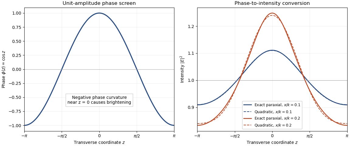
Phase curvature converts a unit-amplitude sinusoidal phase screen into intensity variations; exact paraxial propagation is compared with its quadratic near-screen approximation
. Details. 
Hadamard well-posedness requires existence of a solution for every admissible datum, uniqueness, and continuous dependence of the solution on the datum in the specified normed spaces. An inverse problem is ill-posed if any of these requirements fails. The choice of spaces and norms is part of this assertion: continuity in one norm does not establish continuity in a stronger norm.
For a bounded linear operator , existence requires , and uniqueness requires . Even when both hold for exact data, inversion can be unstable. For example, if but , data approach zero while their solutions do not approach zero. Thus on its range is not continuous. Perturbed data can also leave the range entirely, so an exact solution need not exist after measurement error. These are distinct mechanisms of ill-posedness; the inverse scattering problem below exhibits unstable continuation even on data for which an outgoing continuation exists.
Write , , and choose so that the sphere strictly encloses the scatterer. Normalize the spherical harmonics to be an orthonormal basis of , with surface measure on the unit sphere. The outgoing spherical Hankel function is denoted here by , corresponding to the printed . For fixed , its large-argument behavior isConsequently the coefficient of in the outgoing expansion is asymptotic to : the factors satisfy . With the far-field pattern defined by , we obtainOne can first project onto each spherical harmonic and then take the large- limit. This avoids assuming that the fixed-order asymptotic is uniform in . The Sommerfeld radiation condition selects the outgoing spherical Hankel functions rather than their incoming counterparts.
Let . Its coefficients are , where . Since the field is smooth on a sphere outside the scatterer, ; Parseval's identity givesThe required coefficient condition uses fixed-argument growth of spherical Hankel functions, a different limit from the far-field limit. For fixed ,For completeness, the series of the ordinary Bessel function gives . The identities and give the first formula; the corresponding positive-order series gives the estimate for . The successive series corrections at fixed are . Applying Stirling's approximation to the factorial ratio yieldsIn particular there are positive constants giving upper and lower bounds by the last weight for all sufficiently large . The finite trace norm is therefore equivalent to the spherical far-field range conditionwhere the weight is defined to be one. The same conclusion holds at every larger sphere on which the outgoing field is defined.
The printed comparison with must mean a finite sum: a literal non-strict inequality allows a divergent sum. Also, the supplied one-sided big- bound alone does not imply this necessary condition from a finite trace norm; a lower bound is needed in that direction. The two-sided asymptotic above supplies it. Conversely, its upper bound makes the weighted condition sufficient for an trace at the chosen sphere. This is a condition on exterior-field continuation, not a sufficient condition that the coefficients come from a particular Dirichlet obstacle.
Use the data norm. The coefficients of the measurement error are , so Parseval's identity givesAn unregularized continuation of these measurements to replaces by in the outgoing spherical harmonic expansion. Whenever this continuation has a finite trace, its error isChoose a measurement error supported on a single normalized spherical harmonic, with and all other coefficients zero. The data error has norm exactly , butThis perturbation theory is a finite expansion, so it defines an actual outgoing solution of the Helmholtz equation outside any sphere of positive radius. It is not merely an example of nonconvergent formal coefficients. Taking instead gives data errors tending to zero and trace errors of norm one, which directly proves discontinuity of inversion. General square-summable measurement noise can even violate the spherical far-field range condition, leaving no continuation to the chosen sphere.
For obstacle reconstruction one would continue the field toward the unknown boundary and look for a surface on which , the Dirichlet boundary condition. The unbounded spherical far-to-near-field continuation shows why small far-field errors can cause arbitrarily large errors in the field used to estimate that surface. Locally, a differentiable normal displacement of a candidate boundary must obey the linearized condition . Thus a large continued-field error, or a small normal derivative, defeats an uncontrolled boundary estimate.
There is a necessary qualification to the wording about errors in the scatterer itself. The calculation proves an unbounded field-continuation error. An arbitrary perturbed outgoing field need not correspond to any Dirichlet obstacle, and no admissible class or metric on obstacle shapes is specified. It therefore does not by itself prove an arbitrarily large geometric error in every constrained reconstruction method. Such a claim requires a shape model and an analysis of the boundary-extraction step. The instability displayed here is exactly the mechanism that an unregularized reconstruction must control.
To illustrate Tikhonov regularization precisely, take the unknown to be the trace on a chosen enclosing sphere of radius . Use Hilbert spaces and the forward linear operatorAt real positive , , because the real Spherical Bessel functions have a nonzero Wronskian and cannot vanish simultaneously. Moreover . Thus is an injective compact operator: truncating to finitely many harmonic orders approximates it in operator norm, since the remaining diagonal entries tend uniformly to zero. Its inverse is unbounded. This is a linear field reconstruction; estimating the obstacle from the reconstructed field remains a further nonlinear step.
Given coefficients of measured data , minimize the quadratic functionalVarying in every direction gives . The operator is bounded below by , so it is invertible and the minimizer is unique. In coefficients the minimization is separable: has coefficient and has multiplier . Hence the Tikhonov regularization of spherical far-field continuation isThe implied regularized far-field coefficients are . This suppresses precisely the high-order coefficients that make backward continuation unstable.
Let be the exact trace and , with . The noise-bias decomposition for linear regularization isFor a singular value , the noise multiplier is . Since , its supremum is at most . ConsequentlyThis Tikhonov stability bound measures the trace norm, not a distance between obstacle boundaries. The bias coefficient is times the exact coefficient. It tends to zero for each fixed , is bounded by one, and . Splitting off a finite sum and bounding its tail therefore proves as .
A convergent regularization parameter choice thus satisfiesIn nondimensionalized variables, with is one such rule. Without a smoothness assumption on the exact trace there is no universal bias rate and no universal optimal value of . For a concrete normal-operator source condition, suppose and . Each bias multiplier on is , so . Minimizing the resulting bound gives, for ,This optimizes the displayed worst-case bound under that additional source condition, rather than guaranteeing an exact optimum for every datum.
If only the effect of measurement error is minimized, the multiplier bound decreases when increases. Indeed as . But the reconstruction then approaches zero and its bias approaches . Suppressing noise alone does not optimize reconstruction: must balance noise amplification against regularization bias. A geometrically accurate obstacle estimate additionally needs justified shape constraints and a stable procedure for extracting a boundary from the regularized field.
Articles by others on the same topic
There are currently no matching articles.