Past exam of the mathematics course of the University of Cambridge / 2008 / iii / Paper 41 (Applied Statistics)

Write $q=n-p$. In this normal linear model, the ordinary least squares criterion is $\Vert Y-Xb{\Vert }^2$. Differentiating with respect to $b$ gives the normal equations for linear least squares, $X^{T}Xb=X^{T}Y$. Full column rank of the design matrix makes $X^{T}X$ invertible, and completing the square proves that the unique minimum isSince $\hat{\beta }=\beta +(X^{T}X{)}^{-1}{X}^Tϵ$, its sampling distribution is the multivariate normal distributionLet $H=X(X^{T}X{)}^{-1}{X}^T$ be the hat matrix. It is symmetric and idempotent with rank $p$, and $HX=X$. The regression residual vector is $(I-H)Y=(I-H)ϵ$, soAn orthogonal projection of a Gaussian vector onto the residual space gives $\mathrm{RSS}/{\sigma }^2\sim {\chi }_q^2$. The residual projection and fitted projection have zero cross-covariance, hence are independent because they are jointly normal. In particular, $s^2$ is an unbiased estimator of ${\sigma }^2$ and is independent of $\hat{\beta }$. The maximum-likelihood estimator of ${\sigma }^2$ instead divides by $n$ and is not unbiased.

For the null hypothesis ${\beta }_1=0$, put $v_{11}=((X^{T}X{)}^{-1}{)}_{11}$. Under that null hypothesis, ${\hat{\beta }}_1/(\sigma \sqrt{v_{11}})$ is standard normal and independent of $q{s}^2/{\sigma }^2$. Therefore the Student t-test usesA two-sided level-$\alpha$ test rejects when $|T|>t_{q,1-\alpha /2}$. The denominator is the estimated standard error of the regression coefficient.

The fitted linear regression includes an intercept and three covariates:Thus $n=25$, $p=4$ and the residual degrees of freedom are $21$. The fitted conditional mean isEach slope measures a conditional association with the response while the other two covariates are held fixed. Increasing wind speed by one mile per hour corresponds to a fitted decrease of $0.527410$ in the concentration units used. Its standard error is $0.224904$, giving $t=-2.345$ and a two-sided p-value of $0.0289$: evidence of a negative conditional association at the 5% level. The temperature slope is $0.124991$ per degree Fahrenheit, with standard error $0.075173$, $t=1.663$ and p-value $0.1112$. The insolation slope is $-0.005259$ per langley per day, with standard error $0.006637$, $t=-0.792$ and p-value $0.4370$. Neither of these last two conditional effects is significant at 5%; that does not establish that either true slope is zero. These are associations, not a demonstration of causal effects.

The intercept estimates the mean at zero values of all three covariates. Its value $3.784916$ has a large standard error $7.979647$, giving $t=0.474$ and p-value $0.6402$. The zero-covariate combination may be outside the observed range, so this test may have little practical relevance. Every coefficient test uses a Student t-distribution with $21$ degrees of freedom.

The reported residual standard deviation $s=1.844$ measures unexplained variation in concentration units; the subsequent table gives $\mathrm{RSS}=71.428$, consistent with $s=\sqrt{71.428/21}$ after rounding. The five-number residual summary describes the spread, from $-2.3052$ to $3.4033$, with median $-0.4990$. An intercept forces the residual sum to zero, not the residual median. These five numbers alone cannot establish normal errors, constant variance or independence; residual-versus-fitted and quantile-quantile plots would be more informative, and successive days also warrant checking serial dependence. The coefficient of determination $R^2=0.6533$ means that 65.33% of the sample response sum of squares about its mean is explained by this fit. Its adjusted version iswhich accounts for the number of estimated regression coefficients.

The stepwise selection by the Akaike information criterion searches between the intercept-only model and the specified model with all three main effects. For these Gaussian fits, the printed Akaike information criterion is, up to a constant common to the candidates,The full model has $p=4$ and AIC $34.246$. Removing insolation increases the residual sum of squares by $2.136$ but decreases AIC to $32.982$, so that removal is chosen. Removing temperature or wind instead would give AIC $35.337$ or $38.060$ and is worse. In the next step the candidate models include deletions and restoration of insolation. Keeping wind and temperature has the smallest AIC: removing temperature gives $33.389$, restoring insolation gives $34.246$, and removing wind gives $37.960$. Hence the search stops, givingThe accompanying F-tests compare a larger model with a one-parameter reduction: $F=\Delta \mathrm{RSS}/s^2$, where $s^2$ is estimated from the larger model. For example, removing insolation gives $2.136/(71.428/21)=0.628$, equal to the corresponding squared test statistic. Deletions from the second-stage model use $73.564/22$ in the denominator, whereas restoring insolation uses the full-model denominator. These tests describe the comparisons; they do not determine the AIC choice. In particular, temperature is retained despite its deletion-test p-value $0.15016$. AIC balances fit and complexity, and a stepwise optimum need not be a global optimum over a richer model class. Ordinary coefficient inference after choosing a model does not account for the selection itself.

For positive responses, the Box–Cox transformation is $T_{\lambda }(y)=(y^{\lambda }-1)/\lambda$ for $\lambda \ne 0$, and $T_0(y)=\log y$. Its profile likelihood refits the linear regression and variance at each $\lambda$ and includes the transformation Jacobian. The graph peaks at roughly $\lambda =0.3$–$0.4$. The approximate 95% likelihood-ratio confidence interval contains values a little below zero through approximately one, using the cutoff ${\ell }_{\max }-{\chi }_{1,0.95}^2/2$. Thus a logarithmic transformation ($\lambda =0$) and a square-root transformation ($\lambda =1/2$) are plausible, while leaving the response on its original scale ($\lambda =1$) is at or very near the upper confidence boundary. The broad profile supports considering a mild power transformation; it does not determine a sharply estimated power. The raster does not justify more precise endpoints or a decisive assertion about which side of the boundary $\lambda =1$ lies.

Let $m={\overline{Y}}_{+++}$, $r_i={\overline{Y}}_{i++}$ and $c_j={\overline{Y}}_{+j+}$. The proposed least-squares estimators satisfy the sum-to-zero constraints because ${\sum }_i{r}_i=Im$ and ${\sum }_j{c}_j=Jm$. Define $e_{ijk}=Y_{ijk}-r_i-c_j+m$. Direct summation givesNow write any other admissible parameters as $\mu =m+u$, ${\alpha }_i=r_i-m+a_i$, ${\beta }_j=c_j-m+b_j$, where ${\sum }_i{a}_i={\sum }_j{b}_j=0$. Expanding the ordinary least squares criterion, the cross-products with $e$ vanish by the preceding identities. The cross-products between $u$, $a_i$ and $b_j$ vanish by their zero sums. ConsequentlyEvery added term is nonnegative and all vanish only at $u=0$, $a_i=b_j=0$. This proves the unique constrained minimum, withThe additive-model residual sum of squares and intercept-only residual sum of squares are thereforeThe same orthogonality gives the analysis of variance identityFitting factor B alone yields fitted values $c_j$ and residual sum ${\mathrm{RSS}}_0-S{S}_B$. Fitting A alone gives residual sum ${\mathrm{RSS}}_0-S{S}_A$. Adding B after A then reduces it to ${\mathrm{RSS}}_1$, a reduction of $S{S}_B$ again. The reduction due to B is $S{S}_B$ in either order. This is balanced factorial orthogonality; it generally fails for unequal cell replication.

There are $12$ observations. The additive model estimates $1+(3-1)+(2-1)=4$ independent parameters, so the missing degrees of freedom are A: 2, B: 1, residuals: 8. The individual requested residual sums are below.

To check for an interaction, extend the normal linear model to $\mu +{\alpha }_i+{\beta }_j+{\gamma }_{ij}$, with each row and column sum of $\gamma$ zero. Equivalently, fit the six unrestricted cell means. Its residual sum of squares is the within-cell sumThe interaction adds $(I-1)(J-1)=2$ parameters; the cell-means residual has $IJ(K-1)=6$ degrees of freedom. Under the no-interaction null hypothesis and the independent equal-variance normal error model,The numerator and denominator arise from orthogonal Gaussian projections, proving the exact F-test. Reject for a sufficiently large value. The printed additive analysis of variance table does not supply ${\mathrm{RSS}}_{\mathrm{cell}}$, so it cannot determine this test statistic numerically; the replicated cell data would do so.

The intercept-only residual sum of squares contains both main-effect sums and the additive-model residual: ${\mathrm{RSS}}_0=12.7400+0.4033+2.6867=15.8300$. Its residual degrees of freedom are $12-1=11$.

The additive-model residual sum of squares is the reported residual entry: ${\mathrm{RSS}}_1=2.6867$, with $8$ residual degrees of freedom.

By balanced factorial orthogonality, omitting B adds $S{S}_B$ to the full additive residual: ${\mathrm{RSS}}_{A\text{-only}}=2.6867+0.4033=3.0900$. This model has $3$ parameters and $9$ residual degrees of freedom.

By balanced factorial orthogonality, omitting A adds $S{S}_A$ to the additive residual: ${\mathrm{RSS}}_{B\text{-only}}=2.6867+12.7400=15.4267$. This model has $2$ parameters and $10$ residual degrees of freedom.

A Poisson distribution has probability mass $e^{-\mu }{\mu }^y/y!=\exp \{y\theta -e^{\theta }-\log (y!)\}$, where $\theta =\log \mu$. It is an exponential family with $b(\theta )=e^{\theta }$, mean $\mu$ and variance $\mu$. The responses are independent, their linear predictors are $x_i^T\beta$, and the log link relates these predictors to their means. These are precisely the components of a generalized linear model; the log link is its canonical link function and the dispersion is one.

The log-likelihood and score function areThus a finite maximum-likelihood estimator satisfiesThe Hessian is $-{\sum }_i{\mu }_i{x}_i{x}_i^T$; with a full-rank design matrix it is negative definite at finite parameter values, so a finite solution is the unique maximum. A finite maximum need not exist for every possible response/design combination; the displayed equations describe it when it does exist. If the first component of every $x_i$ is one, the first score equation gives ${\sum }_i{y}_i={\sum }_i{\hat{\mu }}_i$.

The saturated model fits each mean as $y_i$, with the limiting mean zero allowed for a zero count. Subtracting the fitted log-likelihood from the saturated log-likelihood gives the Poisson deviancewhere $0\log (0/{\hat{\mu }}_i)=0$. With an intercept, the sum of the second terms is zero, but retaining them is necessary without that score equation.

Take low pH as a reference level. For group $j$, the model with interaction haswhere $b_i$ is biomass. The additive model sets every ${\delta }_j$ to zero. The interaction model estimates six parameters and the additive model four. In the additive model the log-mean curves are parallel straight lines, while the mean curves are positive exponentials with fixed ratios $e^{{\gamma }_j-{\gamma }_k}$. In the interaction model the log-mean slopes differ, and the mean ratio is $e^{{\gamma }_j-{\gamma }_k+({\delta }_j-{\delta }_k)b}$. The following sketches illustrate common versus factor-specific slopes in Poisson regression; their coefficients are illustrative, not estimates from the data.

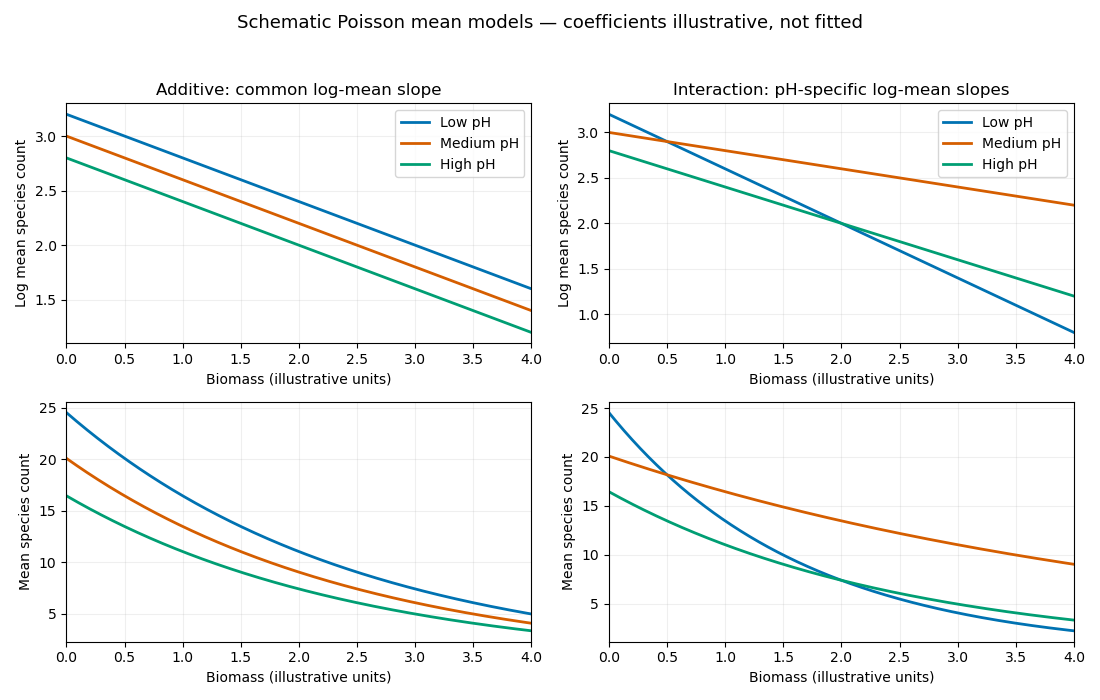
The additive model is nested in the interaction model with two restrictions. The likelihood-ratio test therefore useswhose p-value is $e^{-8}=0.0003355$. There is strong evidence that the biomass slope on the log-mean scale depends on pH. The interaction-model residual deviance $83.2$ is close to its $90-6=84$ residual degrees of freedom, giving no obvious indication of overdispersion from this comparison alone. The supplied deviances contain no slope estimates: they do not establish which pH group has more species, whether each slope is positive or negative, or whether any actual curves cross. Those conclusions require the fitted coefficients and their uncertainty.

The Fort Worth observation for ages 75–84 is missing. It is not a zero count and cannot be replaced by one. The missing cell prevents a direct two-city comparison in that age group and leaves an unbalanced age-by-city table. The youngest groups have only one and four cases, so chi-squared asymptotic approximations to tests and uncertainty may be poor there. The open-ended oldest group and broad age bands can conceal different within-group age compositions between cities.

The denominators are population counts rather than reported person-time, and the observation period is not specified. Comparable coverage, case definitions and time periods must therefore be established before interpreting the numbers as comparable incidence measures. The data contain no information on potential confounders such as individual risk factors or differences in ascertainment. These are aggregated observations on women in the listed ages, and any fitted city association is not automatically causal or generalizable beyond that population.

Index city by $g\in \{0,1\}$ and age group by $j$, with the youngest group the reference level. For each of the 15 observed cells, the grouped-binomial logistic regression assumeswith independent cell counts. The response supplied to R is $C_{gj}/N_{gj}$, and the weights specify the binomial numbers of trials $N_{gj}$. They are not 15 arbitrary precision weights: the conditional variance of the proportion is ${\pi }_{gj}(1-{\pi }_{gj})/N_{gj}$. The logit link models log odds, and the two sets of factor coefficients use corner-point constraints.

There are nine parameters: one intercept, seven age contrasts and one city contrast. Hence the residual degrees of freedom are $15-9=6$, not the total population minus nine. The null model has only an intercept and $14$ residual degrees of freedom. Adding age uses seven more parameters and reduces the binomial deviance from $2330.46$ to $232.28$, a drop of $2098.19$. Adding city then uses one parameter and reduces it by $227.12$ to $5.15$. These are sequential likelihood-ratio tests, asymptotically compared with chi-squared distributions on seven and one degrees of freedom. Both provide extremely strong evidence of an effect; the printed age p-value $0.00$ is rounding, not an exactly zero probability. Because the table is incomplete, sequential main-effect sums need not be invariant to the order of fitting.

The intercept estimate $-11.69364$ is the log odds for the youngest Minneapolis–Saint Paul group. It implies baseline odds $e^{-11.69364}$ and a fitted probability about $8.35\times 10^{-6}$. Its standard error is $0.44923$; its reported Wald test tests log odds zero, or probability $1/2$, rather than a scientifically interesting comparison of groups.

The age coefficients are log odds ratios relative to the youngest group within the same city. Their exponentials are approximately $13.86$, $46.82$, $99.03$, $162.23$, $284.38$, $497.07$ and $484.57$ as age increases through the seven other groups. All these comparisons have large positive Wald statistics and small p-values. Thus the fitted probabilities are much higher in the older groups than in the youngest group. The slightly smaller coefficient in the oldest group than in the preceding group does not itself prove a real decline: that claim needs a contrast and its standard error, including the covariance of the two estimates.

The city coefficient $0.85492$ is the log odds ratio for Fort Worth relative to Minneapolis–Saint Paul, adjusted for age. Its standard error $0.05969$ gives $z=14.322$, so the null city effect is strongly rejected by the Wald test, consistent with the sequential likelihood-ratio test. The fitted constant-over-age city odds ratio and an approximate 95% confidence interval areThis is an odds ratio, not generally a probability ratio. The probabilities here are sufficiently small that the two ratios are close. The absence of an age-by-city interaction is an assumption of the fitted additive log-odds model.

The final binomial deviance is $5.1509$ on six degrees of freedom; its approximate upper-tail p-value is $0.525$. It gives no indication of substantial lack of fit against the saturated observed-cell model. The deviance residuals range from $-1.2830$ to $1.0820$, with median zero and no conspicuously large value in the five-number summary. Neither statement proves that every model assumption holds. In particular, the small case counts motivate checking the accuracy of the chi-squared asymptotic approximation, for example by a fitted-model parametric bootstrap.

The dispersion is fixed at one by the binomial distribution; it was not estimated as a free scale parameter. Four Fisher scoring iterations describe the numerical optimization, not four additional parameters. Residual and cellwise observed-versus-fitted comparisons would help assess adequacy and potential overdispersion.

The second analysis is an exposure-adjusted Poisson regression for case counts:Cell counts are independent, and their conditional variance equals their conditional mean. The population term is an offset with coefficient fixed at one. Thus the fitted case rate is ${\lambda }_{gj}/N_{gj}=\exp ({\alpha }_P+a_{P,j}+{\gamma }_{P}g)$; treating $\log N_{gj}$ as a free covariate would fit a different model. Age multipliers and the adjusted city rate ratio are exponentials of the corresponding regression coefficients.

The fitted model again has nine parameters and six residual degrees of freedom. Sequential additions of age and city reduce the Poisson deviance by $2095.56$ on seven degrees of freedom and $226.52$ on one, respectively. The residual deviance is $5.21$, close to the six residual degrees of freedom. The city likelihood-ratio test is overwhelmingly significant, as in the binomial analysis. The table provides no Poisson coefficient estimates, so an exact Poisson city rate ratio cannot be read from it.

For rare events, $\mathrm{Binomial}(N,\pi )$ is approximately $\mathrm{Poisson}(N\pi )$. The binomial variance is $N\pi (1-\pi )$, close to the Poisson variance $N\pi$, and $\log \{\pi /(1-\pi )\}$ is close to $\log \pi$. Even the largest observed proportion here is below $0.009$. Thus the binomial log-odds model and Poisson log-rate model should give similar fitted counts and tests, as their very similar deviances show.

Both analyses indicate strong age and adjusted city associations, with no apparent large residual lack of fit. The binomial model is natural when each person can contribute at most one case during a fixed period and the denominator counts people at risk. A Poisson count model is natural for event counts with an appropriate exposure or person-time denominator; population size is an approximation to such exposure if the observation periods are comparable. An odds ratio and a rate ratio are different parameters despite being close in this rare-event setting.

The models both assume a common city effect across ages. An age-by-city interaction can be checked by comparing with the saturated model for the 15 observed cells, using the six additional degrees of freedom; the small final deviances offer no substantial evidence against the additive fits in that comparison. This cannot recover the missing city-by-age cell or eliminate unmeasured confounding. Nor is choosing the lower of $5.1509$ and $5.21$ a valid model-selection rule: these deviances are measured against saturated models for different response distributions.

Survival data describe the time $T$ from a specified origin to an event, together with covariates and information about how observation begins and ends. Some event times are observed exactly; others are subject to censoring or excluded by truncation. Here the time origin is the opening of a business and the event is its closure. An observed record contains an entry age, an exit age, an event indicator and the business characteristics. The time origin and observation mechanism are part of the data specification.

With right censoring, an event has not occurred by the last observation time $C$, so the data establish only $T>C$. One records $Y=\min (T,C)$ and $\delta =1_{\{T\le C\}}$, distinguishing an observed event from a censored exit. A business still operating at the follow-up deadline is administratively right-censored. Its observed age is a lower bound on its lifetime, not its eventual closure age. Standard survival analysis requires suitable independent censoring, possibly conditional on the fitted covariates.

With left truncation, a subject is observed only if it survives to its entry time $E$: subjects with $T\le E$ are absent from the sample. A business already operating when observation begins has this delayed-entry mechanism. It joins a risk set only after its recorded entry age. Left truncation excludes earlier failures entirely; left censoring instead includes subjects whose event is known to have happened before a specified time. These mechanisms must not be conflated.

Statistician B uses the more appropriate analysis. Its start–stop representation includes left truncation as well as right censoring. Both entry and exit are ages since opening, so a business belongs to the risk set at age $t$ only when $\mathrm{ageatentry}<t\le \mathrm{obsage}$. The event indicator distinguishes closure from a censored end of observation. The counting-process representation does not mean that multiple closures per business have been observed.

Statistician A records only exit and status and treats every sampled business as at risk from opening. That incorrectly adds already-established businesses to risk sets at ages before they entered observation, ignoring their necessary survival to entry. Its first risk count is $60$, whereas B's is $25$. The extra non-events dilute early estimated closure hazards and here bias the estimated survival upward. Correcting left truncation makes later risk sets capable of increasing as businesses enter at their respective ages.

For the Kaplan–Meier estimator with delayed entry, at event ages $t_j$ with $d_j$ closures and $r_j$ businesses at risk,The standard error follows from the Greenwood formula. Between event times this survival function estimate is constant. At age five the last preceding event is at $4.52$, and at age ten it is at $9.90$. Thus the requested estimates, including their precision, areandThese correspond to estimated proportions 46.2% and 28.0%, not to the probability of surviving five or ten additional years conditional on being sampled at an arbitrary age. A's corresponding estimates $0.650$ and $0.407$ use the inappropriate risk sets.

This interpretation assumes appropriately independent entry and censoring and a suitable common lifetime distribution across entry cohorts. A delayed-entry correction does not remove arbitrary informative sampling or calendar effects. More generally, if no observation covers the earliest ages, absolute survival from opening requires additional information about survival before the first observable age; the reported product-limit normalization is the one used in the supplied analysis.

Converting size to a regression factor allows two unrestricted contrasts rather than imposing a linear trend on numerical size codes. The command relevel with a numeric second argument selects the second existing factor level as its reference level. For sorted codes $0,1,2$ this is medium, coded $1$. However, the displayed coefficient labels size1 and size3 instead correspond to codes $1,2,3$ with code $2$ as reference. The printed coding and coefficient labels are inconsistent. The actual factor levels and labels must be checked. Under the intended medium-size reference, the two reported contrasts compare small and large businesses with medium ones; with literal $0,1,2$ coding their printed names would be size0 and size2.

Using B's delayed-entry survival object, the Cox proportional-hazards model isHere $h_0$ is the unspecified baseline hazard for a medium-size village business and $c$ is the Cambridge indicator. The fitted hazard ratios are conditional on the other covariates and constant over business age under the proportional hazards assumption. The function fits regression coefficients through partial likelihood; its survival object must actually be B's version, rather than A's earlier object with the same name.

The location coefficient $-0.803$, with standard error $0.344$, gives $z=-2.335$ and a two-sided Wald test p-value about $0.02$. Its reported hazard ratio is $0.448$, with 95% confidence interval $(0.228,0.879)$. At the same age and size, a Cambridge business therefore has an estimated closure hazard about 55.2% lower than a village business. The reciprocal ratio is $2.23$. A hazard ratio is not a survival-probability ratio or a proportional increase in lifetime.

The intended small-versus-medium contrast is $-0.322$, with standard error $0.482$, $z=-0.669$ and p-value $0.50$. Its hazard ratio is $0.724$, with 95% confidence interval $(0.282,1.863)$. The intended large-versus-medium contrast is $-0.224$, with standard error $0.375$, $z=-0.598$ and p-value $0.55$; its hazard ratio is $0.799$, with interval $(0.383,1.666)$. Neither size contrast provides convincing evidence of an effect. The wide intervals also show why these results do not establish equality of size-specific hazards.

The sample has $60$ businesses. The likelihood-ratio test, Wald test and score test jointly test all three coefficients being zero; their statistics are $5.45$, $5.76$ and $6.01$ on three degrees of freedom, with p-values $0.142$, $0.124$ and $0.111$. None rejects at 5%. This is compatible with the significant one-coefficient location test: testing a specified one-dimensional contrast and testing three coefficients together are different questions. The location result offers some adjusted evidence, but the joint output does not demonstrate a strong overall improvement, and interpretation should acknowledge the uncertainty and the number of comparisons.

The reported $R^2=0.087$ is a Cox–Snell likelihood pseudo-R-squared, here $1-e^{-5.45/60}\approx 0.087$. It measures likelihood improvement rather than a literal fraction of variance in lifetimes explained. Its attainable maximum is reported as $0.979$. It does not validate the proportional hazards assumption or establish useful predictive performance. Adjusted survival predictions would require estimating the baseline survival function as well: $S(t\mid z)=S_0(t{)}^{e^{{\beta }^{T}z}}$. The coefficient summary alone does not supply adjusted five- or ten-year survival probabilities.

Before reporting results, check the size coding discrepancy, the precise sampling dates and the survival records. The stated January 2000–December 2005 span is six calendar years, despite being called five years. Check nonnegative ages, entry no later than exit, correctly recorded closure indicators and the same opening-based clock throughout. Establish whether inclusion and censoring are plausibly independent of lifetime given the covariates, and whether different opening cohorts or calendar environments can reasonably share the fitted lifetime model. Simply including delayed entry does not cure informative selection, omitted confounders or dependence between businesses.

Assess proportional hazards using Schoenfeld residuals against time and a proportional hazards assumption test, supplemented by groupwise log-minus-log survival plots. Investigate influential observations with coefficient-deletion diagnostics and deviance residuals, and inspect overall fit using Cox–Snell residuals. Consider a city-by-size interaction or time-varying effects if supported by the available events, rather than relying on the displayed three main effects. Finally, report the uncertainty and declining late risk sets—only six remain at the final listed event—and distinguish a conditional association from a causal explanation or a prediction for all future businesses.