The empirical distribution function isIf is a standard Brownian motion on , the standard Brownian bridge is . It is a centred Gaussian process with continuous paths, endpoints zero, and covarianceThe F-Brownian bridge is the time-changed Gaussian process . Its covariance is , exactly the covariance of the empirical distribution process .
The Donsker theorem for empirical distribution functions states that for every cumulative distribution function ,Thus this is a function-space central limit theorem, not merely convergence of each finite collection of evaluations. The limit is a tight centred Gaussian process. No continuity of is required for this statement; a jump of can give a jump of .
For precision, is generally nonseparable, and the finite-sample process need not be a Borel-measurable random element for its norm topology. The displayed convergence in distribution has the usual empirical-process interpretation: for every bounded continuous real functional , the outer expectation and inner expectation of converge to . The outer expectation is the infimum of expectations of measurable majorants, and the inner expectation is its negative applied to . For measurable real statistics this gives ordinary convergence in distribution. The limit is tight and separably supported: maps the separable space of continuous bridge paths continuously into .
The map is Lipschitz, sinceConsequently the continuous mapping theorem applied to the Donsker theorem for empirical distribution functions gives . The statistic on the left is measurable: both and are right-continuous, so its supremum equals the supremum over rational .
If is continuous, its limits at and are zero and one. The intermediate value theorem therefore shows that contains , even when is not strictly increasing. A continuous Brownian bridge is zero at its endpoints, so pathwiseWe obtain the Kolmogorov-Smirnov theorem in the required form:Continuity of is what makes the limit independent of the unknown cumulative distribution function.
Choose with . The law of has no atoms. For example, the Brownian reflection principle and conditioning a Brownian motion on its endpoint give for : the reflected endpoint density at zero is the normal density at , divided by its value at zero. Hence both one-sided maxima have continuous laws, and an atom of would require an atom of one of them. Also , since is nondegenerate. Thus such quantiles give the desired limiting coverage.
An asymptotic simultaneous confidence band isIndeed, because , the event that for every is precisely . Its probability tends to . This is simultaneous coverage over all real , rather than separate pointwise confidence intervals.
For a kernel for density estimation and smoothing bandwidth , the kernel density estimator isWe use the convention that a kernel of order ell hasThe kernel for density estimation is integrable and can have negative values; requiring nonnegativity would prevent its second moment from vanishing. Some conventions additionally require a nonzero moment of order . The construction below covers that convention too.
The Legendre polynomial kernel construction uses the polynomial reproducing kernel at zero:Every polynomial of degree at most has the expansion , since the displayed Legendre polynomials have those successive degrees and form an orthonormal basis of this polynomial space. ThereforeTaking proves all the required moment identities. Boundedness and compact support give every absolute moment and a finite L2 norm. If a nonzero moment of order is required, replace this kernel byThe lower moments are unchanged by orthogonality. If , then because otherwise would lie in the polynomial space of degree at most . Evaluating its full Legendre expansion at zero gives , so .
For instance, a simple kernel satisfying the moment conditions needed for three derivatives isIts negative wings cancel its central contribution to the second moment.
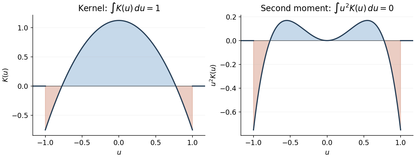
Signed kernel and cancellation of its second moment
. Details. 
Here is the third-order pointwise kernel error bound. Write and , and use any square-integrable kernel with unit integral, first two moments zero and . A change of variables givesBy the Taylor theorem with Lagrange remainder,The moment cancellations consequently give the uniform bias of a kernel density estimator boundFor the variance, independence and another change of variables giveThe triangle inequality and Cauchy-Schwarz inequality now yieldBalancing against givesThe constant is independent of both and . The original PDF has exponent ; the converted TeX's is a transcription error.
To obtain the final parametric rate, we choose a flat-top kernel for density estimation. This kernel also satisfies all the preceding moment conditions, so a single kernel works for both constructions, with different bandwidth choices. With the Fourier transform convention , choose a real even function equal to one on and zero outside , and putSuch a cutoff is explicit: if for and zero otherwise, take . It is constant near zero, and its endpoint transitions are smooth. Repeated integration by parts shows that and all its derivatives decay faster than every power, so lies in the Schwartz space. The Fourier inversion and moment differentiation of the Fourier transform giveThus this kernel can be used with for the preceding general bound.
For the sharper example choose the probability density functionTo check this is a density and identify its Fourier transform, direct integration givesThe continuous value at zero is as displayed. This function is nonnegative and integrable, being bounded near zero and at infinity. Fourier inversion gives , and in particular . Differentiation of this compact frequency integral also shows that and are bounded. Since on the support of , the convolution theorem givesBoth sides are continuous, so the equality holds at every . There is therefore exactly zero bias of a kernel density estimator at bandwidth one, and the variance bound above givesThis is parametric-rate kernel estimation of a bandlimited density. A fixed bandwidth is appropriate because it reproduces this particular density exactly; a generic density would retain a nonzero smoothing bias.
For an orthonormal wavelet construction, setThe scaling function generates the approximation spaces , while generates the detail spaces in the multiresolution analysis, with . At coarse resolution zero, the family is an orthonormal basis of .
For the given square-integrable function the coefficients and wavelet series areFor real wavelets these are the real L2 inner products; use complex conjugates for a complex basis. The series converges in the L2 norm, and its coefficients satisfy the Parseval identity for a Hilbertian basisAn hypothesis alone does not assert pointwise convergence.
The resolution- wavelet projection is the orthogonal projection onto :The two expressions coincide by iterating . Orthogonality gives , which tends to zero. One can equivalently write the projection with kernel , interpreted as the same orthogonal projection.
In fixed-design nonparametric regression, the observations satisfywith independent errors. In the usual Gaussian version . The regression function is evaluated at the design sites, so it must be specified pointwise there, not only as an equivalence class. For , the observations concern on . They cannot identify its values outside this interval. Use an interval-adapted wavelet basis on , consisting of coarse functions and detail functions ; a Haar wavelet basis is one explicit choice.
Here is a wavelet regression estimator valid for every . Divide into cells , with the value at zero assigned arbitrarily, and form the observed step function on . For any normalized basis function , estimate its coefficient byThe wavelet regression estimator at resolution is thereforeOnly finitely many interval basis functions occur. Its expectation is , where equals on . Thus approximation of includes the resolution bias and the grid discretization bias. For continuous , the latter tends uniformly to zero by uniform continuity. No smoothness or consistency claim for arbitrary pointwise representatives of functions is needed to define the estimator.
The common point-evaluation version replaces each weight by , givingThese are Riemann-sum approximations to the coefficient integrals. For Haar wavelets, , and , they equal the integrated-weight coefficients exactly if the dyadic cells and pointwise basis versions are chosen right-closed. Each retained basis function is then constant on every sampling cell. This gives a concrete implementation by the discrete wavelet transform. A sensible finest resolution has ; beyond the grid scale there are details the data cannot resolve.
For wavelet coefficient thresholding, retain the coarse coefficients but discard detail coefficients dominated by noise. A hard-threshold version isAlternatively, soft thresholding replaces each detail coefficient by . The unthresholded wavelet regression estimator retains all details at the chosen resolution; thresholding retains evidence for local features while suppressing small fluctuations.
The thresholds can be derived from a simultaneous wavelet coefficient noise bound. Write . Independence giveswhere the inequality applies the Cauchy-Schwarz inequality on each cell of length . In the dyadic Haar implementation, exactly. For Gaussian errors, the normalized coefficient noise is standard normal. More generally, independent centred sub-Gaussian random variables with parameter giveIf detail coefficients are considered, a union bound consequently justifiesWith probability at least , every retained detail's noise is below its corresponding threshold; independence between the coefficient errors is unnecessary. With of order and , these thresholds have the familiar order . Coefficients larger than their noise level represent potential signal, and a coefficient zero in the discretized mean is not selected on this simultaneous event. If is unknown, a consistent noise-scale estimate can be substituted; for Gaussian errors and predominantly negligible finest-level signal, the median absolute finest-level coefficients divided by the standard-normal absolute median estimates . Without a Gaussian or sub-Gaussian tail assumption, finite variance alone does not justify the logarithmic thresholds: Chebyshev inequality and the union bound instead permit .
A real functional is Hadamard differentiable at if there exists a continuous linear functional such that, whenever , and in the normed vector space,If is defined only on a subset, require to lie in its domain. The variation of the directions is essential: convergence along each fixed direction alone is a weaker differentiability condition. Tangential Hadamard differentiability restricts the limit directions to a specified subspace; here the derivative is defined on all of .
We prove the functional delta method using compact sets, so do not need an unjustified application of the Skorokhod representation theorem on an arbitrary nonseparable normed vector space. As usual for function-space convergence in distribution, the limiting random element is tight, and the real statistics are measurable, or convergence is understood through outer expectations. These are automatic under the usual separable complete random-element formulation; the empirical-process formulation used below has a tight separably supported limit.
For putHadamard differentiability says for every convergent sequence of directions, since continuity gives . It implies a Hadamard remainder near a compact set: for every compact and there are and such thatTo prove it, suppose it failed. Choose and at distance less than from with . Choose with . A subsequence of converges by compactness, so the corresponding converge too. The defining derivative limit contradicts the lower bound on .
Now let and . Given , tightness of a probability measure provides a compact with . For the open -neighbourhood , the Portmanteau theorem givesOn the preceding uniform remainder is less than for all sufficiently large . Consequently . Since is arbitrary, this remainder tends to zero in probability. We have proved the actual expansionContinuity of and the continuous mapping theorem give . The vanishing remainder and Slutsky theorem therefore yieldThis derivation uses the derivative definition, rather than assuming a uniform Fréchet remainder over every bounded set. If outer expectations are needed, the same compact-neighbourhood argument uses outer probabilities and gives the corresponding empirical-process functional delta method.
For the statistical application, use the sample's empirical distribution function and the plug-in estimatorHere the printed denotes bounded pointwise functions with the supremum norm, namely , rather than equivalence classes modulo Lebesgue null sets. Assume Hadamard differentiability at the true and the usual measurability of the scalar estimator. The Donsker theorem for empirical distribution functions and the proved functional delta method giveNo continuity of is needed for this application. Since the derivative is continuous and linear and the bridge is a centred Gaussian process, is a centred Gaussian real random variable, possibly identically zero.
Finally, a finite real weak limit ensures the required boundedness in probability. Choose so large that . Applying the closed-set part of the Portmanteau theorem to givesHence there is such that, for every ,In particular the upper-tail condition in the question holds. The plug-in estimator has estimation error , even when its limiting variance is zero.
Articles by others on the same topic
There are currently no matching articles.