Let denote the fluid pressure perturbation divided by the reference mass density, and let be the buoyancy perturbation. The buoyancy frequency satisfies . Linearization requires small boundary slope , small displacements compared with the vertical scales of the disturbance and background, and advection small compared with the oscillatory acceleration. For a propagating internal gravity wave this includes ; boundary slope alone is insufficient when . The Boussinesq approximation also requires small relative mass density differences over the region of interest. These conditions must hold for the resulting disturbance, including any amplification by resonance.
The inviscid Linearized Boussinesq equations and linear kinematic boundary condition areWrite the velocity field as . Incompressibility and horizontal momentum balance giveThe vertical momentum balance therefore yieldsFor a real vertical wavenumber , this gives the dispersion relationWhen , define . The radiation condition selects , because energy must leave the boundary upward. The boundary-forced internal gravity wave isIts wavevector is , its phase velocity is , and its group velocity isThus the phase velocity points down and right, while the group velocity points up and right. They are perpendicular. Internal-wave polarization makes the particle motion an oscillation along the group velocity direction, with zero first-order mean transport. The constant-phase lines of an internal gravity wave are also parallel to the group velocity. Their inclination above the horizontal satisfies .
When , set . Boundedness at infinity selects the evanescent waveThe horizontal and vertical velocity components are in quadrature: fluid particles describe small ellipses, and the response decays over . There is no upward time-averaged energy flux, because and are in quadrature. A real vertical group velocity is not defined for this evanescent wave. The pattern travels horizontally with phase velocity .
For the response is the evanescent wave with ; the ratios should not be used. At the cutoff , the bounded harmonic solution has , : it neither decays nor has nonzero upward group velocity. It is the limiting cutoff response, rather than a localized radiating disturbance. A uniform nonzero buoyancy frequency in an infinitely deep Boussinesq approximation is itself a local idealization of the background mass density.
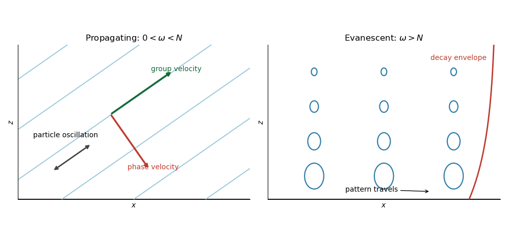
The arrows distinguish the phase velocity, group velocity, and oscillatory particle motion of the internal gravity wave. The right panel shows the decay envelope and particle ellipses of the evanescent wave.
At the change in buoyancy frequency, continuity of vertical velocity and fluid pressure givesThe background mass density is continuous, so there is no interfacial density jump or separate surface restoring force. Since , these internal-wave transmission across a stratification step conditions are continuity of and . The buoyancy perturbation need not be continuous, because the background density gradient jumps.
Let and . The lower unstratified layer obeys and the upper radiation condition givesPropagating these matching data downward givesThe kinematic boundary condition at the moving lower boundary therefore givesThe upper vertical-displacement complex amplitude at isIn particular, . The unstratified layer attenuates and phase-shifts the transmitted internal gravity wave. The matching height is in the original PDF; the TeX transcription's is a typo.
The central stratified layer supports upward and downward internal gravity waves, whose counterpropagating components form a standing wave. The unstratified regions support evanescent waves, and the upper disturbance decays as . Consequently the central layer is a stratified internal-wave guide, rather than a source of propagating energy at infinity.
The largest response occurs at its trapped normal mode frequencies. They can be specified without solving the forced problem. Set the boundary forcing to zero to find a free normal mode. The lower solution is proportional to , so continuity of fluid pressure and vertical velocity givesIn the central layer writeThe upper Robin boundary condition then gives the exact trapped-mode conditionThe left side increases strictly from zero to infinity, so there is one positive root for each ; the frequencies accumulate at zero. This is constructive phase matching after reflection at both ends. The phase shifts from the evanescent waves matter: simply imposing integer half-wavelengths across the stratified layer is generally incorrect.
In the ideal inviscid model, exact resonant forcing has no bounded steady harmonic solution. The undamped normal mode grows secularly under sustained forcing. Weak viscosity or other losses would produce large finite peaks near the displayed frequencies; the linear approximation eventually fails if the disturbance becomes too large.
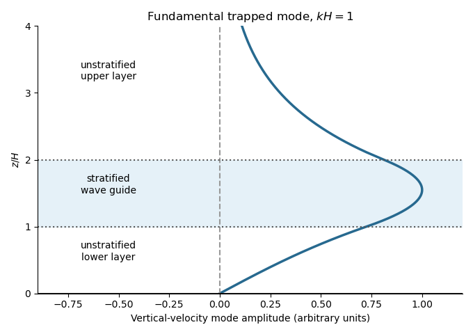
A trapped internal-wave mode
. Details. The illustrated free normal mode has an oscillatory central region and evanescent wave tails. Its lower tail reaches the fixed zero-displacement boundary; its upper tail decays to infinity.
The exact mixture equation of state is . Keeping first-order terms in the small particle volume fraction and thermal expansion givesThe omitted term is . The downward solid-volume particle deposition flux is ; the corresponding particle mass flux is . Uniform vertical mixing and constant layer depth implyFor , set . Thenand henceThe heated particle-laden layer loses its stable density stratification when this contrast vanishes. For , solving for the neutral-buoyancy time givesThe layer is neutral at and statically unstable for . The subsequent uniformly mixed lower-layer solution cannot represent the resulting overturning.
If , then , , and the continuous limit is . If , the layer stays denser than its surroundings at every finite time and becomes neutral only asymptotically when ; thus . These limiting cases must replace the printed formula when its denominator vanishes.
Use the shallow-water approximation, a hydrostatic vertically mixed layer, a deep motionless ambient, and no ambient fluid entrainment. Particle loss changes reduced gravity but changes total layer volume only at the discarded dilute-particle order. Likewise thermal expansion changes the equation of state while the leading Boussinesq approximation retains volume conservation. DefineDepth integration of mass conservation, horizontal momentum balance, particle transport, and the heating law givesHere the integrated excess hydrostatic pressure is . There is no particle source from the bed. Bed drag and the particle contribution to inertia are neglected at this order. The equivalent variable-buoyancy shallow water equations areThe term is necessary when heating or particle loss makes the reduced gravity vary horizontally.
For , the quasilinear system hasIts characteristic polynomial factors asThus the characteristic curves have slopesOn the two repeated contact characteristic curves, the particle and heating laws are and . Writing and , the gravity-wave compatibility relations areFor and , gravity-wave right eigenvectors can be taken as . The contact eigenspace has dimension two: and , with independent . Therefore has a full set of real eigenvectors.
The system is hyperbolic throughout strict static stability, but not strictly hyperbolic because the contact speed is repeated. At the eigenvalues coalesce and this diagonalizability is lost; when the gravity-wave speeds become complex, reflecting the loss of a statically stable lower layer.
Let be the layer volume per unit transverse width. The gravity-current box model imposes ; it approximates the front and scalar balances, rather than an exactly uniform solution of the local momentum equation. For a specified constant front Froude number , the heated particle-laden gravity current satisfiesThe initial data are , , and . The gravity-current front condition applies only while .
For heating without settling, and . Integration of the front equation givesHence the heated gravity-current runout isIt is reached at the neutral-buoyancy time within this front model. A finite-momentum current could subsequently coast or lift off: the formula is the maximum predicted by the prescribed gravity-current front condition, which contains no independent front inertia.
For settling without heating, . Set , so . Eliminating time yieldsThus the runout length of a gravity current isThis length is approached as , because positive concentration cannot disappear at a finite time under the settling law. If distance means displacement from the removed barrier, the answer is in either case.
It is important to fix the mass flux convention. With literal mass units and the corresponding density-weighted buoyancy flux, the Boussinesq approximation and circular top-hat plume model giveReplacing by in inertial fluxes is the Boussinesq approximation; the density difference is retained in the buoyancy flux. Define the kinematic plume fluxesIf the symbols instead denote the customary kinematic fluxes, simply omit the factors in all conversions below. Keeping the two conventions consistent is essential for the jet length and dimensional prefactors.
The Batchelor entrainment hypothesis prescribes inward edge velocityThe constant entrainment coefficient relates ambient inflow to the local axial velocity. A centreline segment of arc length entrains volume . Hence, setting ,The buoyancy flux is conserved because the homogeneous entrained ambient has zero density deficit, and mixing has no buoyancy source or sink. The imposed zero source mass flux with nonzero source momentum flux is a singular point-source idealization, not a finite-radius nozzle with zero emitted fluid. Indeed and the plume reduced gravity diverge as with nonzero source fluxes. The Boussinesq approximation cannot remain valid arbitrarily close to that point. The top-hat plume model is applied outside the unresolved source region.
For a neutrally buoyant horizontal turbulent round jet, a segment's horizontal momentum flux changes only if an external horizontal force or ambient momentum input exists. Neither is present, soPositive buoyancy adds a vertical force, not a horizontal one. Therefore remains true for an inclined forced plume even when ; in general .
The net upward force on a segment is . Since and , vertical momentum balance givesIn kinematic plume fluxes, the equations are , , where . The centreline geometry satisfiesFor , beyond the source, and an initially nonvertical turbulent round jet pointing right, increases and the centreline turns toward the vertical. The magnitude of momentum flux is not conserved once the tangent has a vertical component.
Put and under the literal mass convention. Their dimensions are and . Dimensional analysis givesThe jet length compares source momentum with buoyancy. The region near the source behaves as a turbulent round jet; sufficiently far away, the forced plume behaves like a pure plume. With the constant entrainment coefficient retained explicitly, substantial turning occurs over a length of order , where . Statements involving or normally hold this dimensionless coefficient fixed.
Near the point source, and the Batchelor entrainment hypothesis gives . ThereforeIntegrating the centreline tangent givesTo leading order the centreline is a straight turbulent round jet at its source inclination. For the horizontal source, the first curvature is the horizontal forced-plume trajectoryFor a vertical source, , the trajectory stays vertical rather than developing this cubic transverse displacement. If , there is no finite buoyancy-induced jet length and the turbulent round jet remains straight.
For a horizontal source, throughout. Far downstream , so the kinematic plume fluxes obey the vertical pure plume equations to leading order,Set and with . Matching exponents and coefficients gives and . Consequentlyand the requested literal mass and density-weighted buoyancy fluxes areto leading order. The radius is and the axial velocity decreases as .
The centreline becomes nearly vertical but retains finite horizontal drift:Since , there is a finite positive geometric deficit , and . The equivalent vertical plume virtual origin is therefore located atFor the horizontal point-source forced plume, the virtual source is downstream and below the actual source. The horizontal turbulent round jet first entrains substantial ambient fluid while rising only a little. Thus at the height where it turns upward it already has a finite radius and volume flux; an equivalent pure plume must have begun rising from below to acquire these. The turning displacement, entrained radius divided by its far-field spreading angle, and virtual vertical depth all scale asAt fixed entrainment coefficient this is simply . The arclength origin should not be interpreted as a physical height: the curved near field supplies the additional shift . The numerical constants depend on the chosen top-hat plume model and entrainment coefficient; scaling does not fix them.
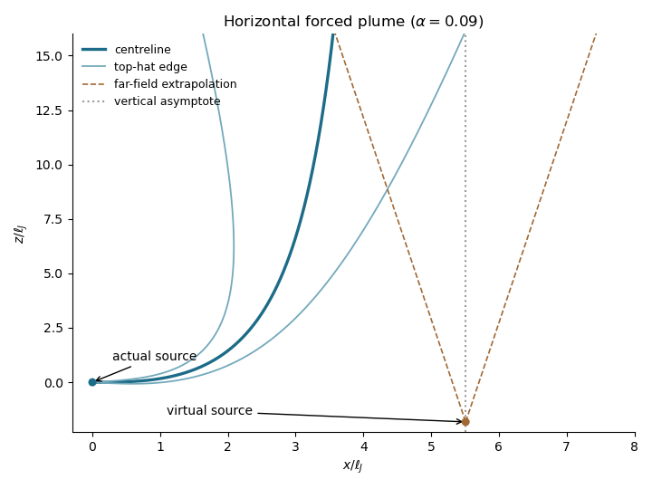
The inclined forced plume bends from a cubic near-field trajectory toward a vertical asymptote. Dashed far-field spreading lines extrapolate to the equivalent plume virtual origin; the marked location is obtained from the integral model for this illustration, not a universal numerical prediction.
Let . A spherical grain has submerged weightNeglect lift and contact torque, and use a sliding static friction model with normal reaction . The inertial quadratic drag iswhere the last equality fixes the convention . Equivalently is the bed shear velocity and is an effective drag coefficient referred to it. A literal grain-level flow speed can differ from the shear velocity; that conversion must then be absorbed into .
Downstream sliding begins when . Defining the Shields parameter by , the threshold force balance isThe grain moves downstream above this threshold in the stated sliding model. Real grain motion can instead involve lift, rolling, irregular contacts, or viscous drag; the printed constant belongs to the particular inertial-drag convention and force balance above.
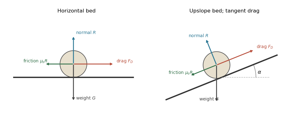
Grain force balances on horizontal and inclined beds
. Details. The normal contact force and resisting static friction balance the drag force and submerged weight at impending motion. The right panel uses locally bed-tangent drag force.
Use locally bed-tangent drag force, consistent with interpreting as bed shear stress. Let the bed rise downstream at angle and retain the same effective drag coefficient. The normal reaction is , while the opposing downslope component of submerged weight is . At impending upslope motion,Thus the inclined-bed sediment threshold isFor ,An uphill slope increases the sediment entrainment threshold; a downhill slope lowers it, until spontaneous gravity-driven motion invalidates the resting-bed model.
There is a geometric convention to specify: if the drag force remains horizontal while the bed tilts, then . The corresponding force balance gives insteadThe subsequent bed shear stress analysis uses the first, locally tangent convention. The two interpretations should not be mixed.
The Exner equation is solid-volume mass conservation: a downstream increase in sediment transport flux removes material and lowers the bed. The factor converts bed-height change into solid-volume change. The saturation length equation models downstream adjustment of actual sediment transport to the equilibrium sediment flux. Grain acceleration and entrainment/deposition need a finite distance, so lags . The last relation is an empirical transport law above the sediment entrainment threshold, with and normally ; below threshold it must be interpreted with a positive part rather than raising negative excess stress to an arbitrary power. It is a constitutive closure, not a consequence of mass conservation.
Take the physical parameters , , and . Linearize about a horizontal, uniformly transporting bed with and . Set and use the real parts ofThe locally planar approximation uses the small instantaneous bed slope to compute the inclined-bed sediment threshold. Since ,A sinusoidal disturbance has both uphill and downhill slopes: the printed describes the uphill derivation, and its first-order continuation applies to both signs. The zero-slope reference is the one implicit in the printed decomposition with constant term ; a finite mean inclined bed would require a shifted base threshold.
A fluid-dynamical shear-response closure is missing from the printed question. The three sediment equations and local slope correction do not determine from . Write the general bed shear response as . A frequently used scale-invariant closure for isHere is the component in phase with bed height and represents an upstream phase lead in bed shear stress. They require an independent flow model and can depend on . Introducing them explicitly makes the linear stability analysis complete conditional on a specified flow response; it does not turn them into data supplied by the question. An example of this hydrodynamic closure is given in Fourrière, Claudin and Andreotti's bedform-instability analysis.
Eliminate the transport amplitudes in the linear stability analysis. For a general bed shear response , the dispersion relation isThis is the most specific result available without adding the missing hydrodynamic closure. With , setMultiplication by gives the growth rate and migration velocityThe packed-bed volume fraction cancels. For a real physical closure the negative wavenumber response is the complex conjugate; the displayed formulas cover the independent normal modes.
If , are treated as constants, the upstream shear stress phase lead promotes growth, while the inclined-bed sediment threshold reduces it and the finite saturation length delays sediment transport. There is an unstable band precisely when : . Within this band , so the growing bedforms migrate downstream. The fastest normal mode satisfiesThis last maximization assumes constant ; if the hydrodynamic coefficients vary with wavenumber, their derivatives also enter the selection condition. When and , all nonzero normal modes decay.
Just above the sediment entrainment threshold,Thus the common regime is stable near onset: the slope penalty overwhelms the hydrodynamic phase lead. This conclusion is conditional on that inequality, not universal. For constant , instability begins only when as well as . The transport sensitivity vanishes at onset for , is finite for , and is singular for . Exactly at threshold, the positive-part transport law needs separate treatment; the above linearization with perturbations small compared with is unavailable.
Far above the sediment entrainment threshold, . If , the unstable cutoff tends to , and the dominant wavelength is set by the saturation length. Both growth rate and migration velocity scale with , apart from their length factors. Their numerical values and any detailed dependence on wavenumber still require a flow closure.
For example, prescribing uniform shear stress independently of the bed gives andThis equally admissible closure illustrates why instability cannot be asserted from the printed sediment equations alone.
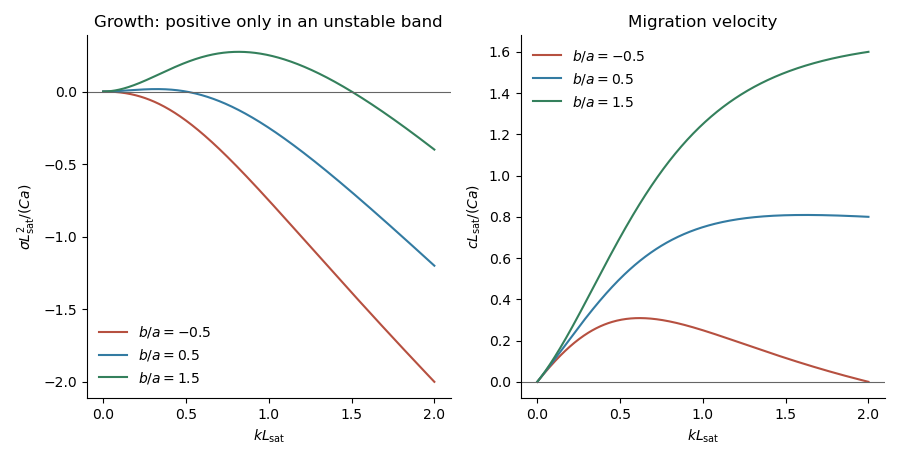


The plots use constant and three illustrative ratios . They show how the sign of the shear phase lead minus the slope correction determines stability; they are not numerical predictions for unspecified flow conditions.
Articles by others on the same topic
There are currently no matching articles.