Drag (physics)

A drag force opposes an object's motion relative to a surrounding fluid and transfers momentum between them.

Linear drag opposes the velocity relative to the surrounding medium with magnitude proportional to its speed, where $\alpha >0$. Its power is ${\mathbf{F}}_d\cdot \mathbf{v}=-\alpha |\mathbf{v}{|}^2$, so it dissipates kinetic energy. Under a constant external force, the resulting linear ordinary differential equation relaxes exponentially on the time scale $m/\alpha$.

When momentum relaxes much faster than the imposed motion, force balance replaces the inertial equation: $\zeta \dot{x}=F(x,t)$ in a deterministic one-dimensional model. The linear friction coefficient sets the time scale. Thermal forcing, if included, gives overdamped Langevin dynamics.

The dimensional linear friction coefficient relates drag force and velocity, $F_d=-\zeta v$, and has units of force divided by speed. It differs from the dimensionless aerodynamic drag coefficient. For an isolated sphere in Stokes flow, the Stokes drag law gives $\zeta =6\pi \eta a$.

For constant downward gravitational acceleration $g$ and linear drag $-\alpha v$, the upward velocity solves $m\dot{v}=-mg-\alpha v$ with $v(0)=u_0\ge 0$. Its first zero occurs at the displayed time. The dimensionless control variable is $\alpha u_0/(mg)$, and the limit $\alpha \to 0$ gives $u_0/g$.

The drag coefficient measures a drag force against a specified scale of force. Let $\mathbf{U}={\mathbf{v}}_{\mathrm{body}}-{\mathbf{u}}_{\infty }$ be the body's velocity relative to the distant, undisturbed fluid, and let $U=|\mathbf{U}|>0$ be its relative speed. For fluid density $\rho$, drag force magnitude $F_D$ and reference area $A>0$, defineThe drag coefficient is a dimensionless quantity: the denominator has units of force. The reference area must be reported with it. For a sphere of radius $a$, the usual choice is the frontal area $A=\pi a^2$. Choosing its entire surface area $4\pi a^2$ instead divides the reported drag coefficient by four for the same physical drag force. Comparing coefficients without comparing their reference areas can therefore be misleading. ^[ref]

For a rigid sphere in steady flow through an unbounded Newtonian fluid with constant dynamic viscosity $\mu$, incompressible flow and the no-slip boundary condition, the creeping-flow limit requires the diameter-based particle Reynolds number ${\mathrm{Re}}_d=2a\rho U/\mu \ll 1$. The Stokes drag law gives $F_D=6\pi \mu aU$. Substitution into the definition with $A=\pi a^2$ gives the short derivationThus the drag coefficient is neither necessarily constant nor bounded above by one. The formula containing $U^2$ still describes linear drag here, because the drag coefficient varies as $1/U$. The relation $C_D=24/{\mathrm{Re}}_d$ is the leading small-Reynolds number approximation, not a measured curve valid at every Reynolds number. ^[ref]

For a worked example, stipulate dynamic viscosity $\mu =0.10\mathrm{Pa}\mathrm{s}$, density $\rho =1000\mathrm{kg}{\mathrm{m}}^{-3}$, radius $a=10^{-4}\mathrm{m}$ and relative speed $U=10^{-3}\mathrm{m}{\mathrm{s}}^{-1}$. Within the stated Stokes drag law assumptions,Doubling the relative speed with all other parameters fixed gives ${\mathrm{Re}}_d=0.004$ and $C_D=6000$: the predicted drag force doubles to $3.76991118\times 10^{-7}\mathrm{N}$. Falsely holding the drag coefficient at $12000$ would instead quadruple the drag force. Both particle Reynolds numbers remain small, so the comparison is within the creeping-flow approximation.

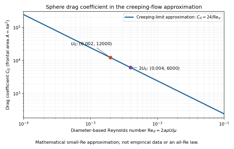
The useful idea is to separate the force scale from the dependence on geometry and flow conditions. A drag coefficient can help compare experiments, but changing Reynolds number can change the coefficient itself; NASA Glenn explicitly stresses matching the relevant flow conditions. The elegant cancellation above also exposes a common mistake: a drag coefficient definition does not by itself impose a quadratic drag law.

Quadratic drag has magnitude proportional to the square of the relative speed and points opposite to the relative velocity.

For an isotropic model of a body of fixed shape, let $\mathbf{U}={\mathbf{v}}_{\mathrm{body}}-{\mathbf{u}}_{\infty }$ denote its relative velocity through the distant fluid, with $U=|\mathbf{U}|$. A constant positive resistance $k$ givesHere density $\rho$, reference area $A$ and drag coefficient $C_D$ are held fixed over the modeled range of relative speeds. The vector formula makes the direction explicit: the drag force on the body opposes its motion relative to the fluid, and vanishes at $U=0$. For a general body, orientation and other flow conditions can affect the drag coefficient; treating it as a constant requires a regime in which that is an adequate approximation. ^[ref]

Compare two distinct models at a chosen relative speed $U_0>0$. A linear drag model has $F_D(U)/F_D(U_0)=U/U_0$, while a constant-coefficient quadratic drag model has $F_D(U)/F_D(U_0)=(U/U_0{)}^2$. At $U=2U_0$ their drag force ratios are two and four respectively.

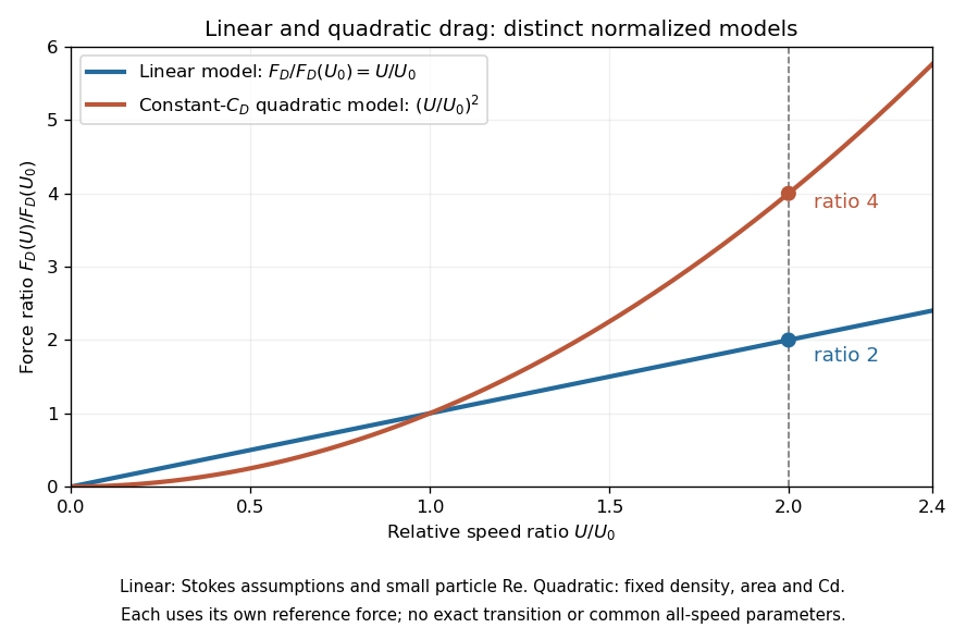
This distinction matters when estimating terminal velocity or trajectories such as descent from rest under quadratic drag: doubling relative speed increases the resistance much more strongly in the quadratic drag model. An approximately constant drag coefficient can occur in another Reynolds number regime; its use must be justified there. Conversely, substituting the creeping-flow sphere coefficient $C_D=24/{\mathrm{Re}}_d$ into $F_D=\frac{1}{2}\rho U^{2}A{C}_D$ recovers linear drag, so writing this general formula does not make the resistance quadratic. Neither approximation should be extended across all Reynolds numbers.

The distinction already appears in the original investigation underlying the Stokes drag law, read on 9 December 1850: article 42 identifies resistance proportional to relative speed and distinguishes it from a contribution proportional to the square of relative speed. ^[ref]

For positive downward speed, gravity and quadratic drag give $m\dot{v}=mg-\alpha v^2$, $v(0)=0$. Separation and the integral of $(1-s^2{)}^{-1}$ give the displayed approach to terminal velocity. The fallen distance is $(m/\alpha )\log \cosh (\sqrt{\alpha g/m}t)$. The limit as $\alpha \to 0$ recovers $v=gt$ and distance $g{t}^2/2$.

For an ice mass in still water, approximate the wind stress by a fixed vector $a{\mathbf{e}}_x$ while retaining quadratic drag in the water. With mass per water-drag area $\mu =m/A_w$, water coefficient $b={\rho }_w{C}_w$ and $f=2\Omega \sin \varphi$, the steady balance is $a{\mathbf{e}}_x=bU\mathbf{u}+\mu f\hat{\mathbf{z}}\times \mathbf{u}$. Resolving along the drift and perpendicular to it gives $a\cos \theta =b{U}^2$, $a\sin \theta =\mu |f|U$. Thus $b^2{U}^4+(\mu f{)}^2{U}^2=a^2$ and $\tan \theta =\mu |f|/(bU)$. The direction is right of the wind in the northern hemisphere and left in the southern hemisphere. This angle neglects intrinsic boundary-layer turning, ocean currents and contact forces; it is not a universal observed sea-ice turning angle.

The normalization $\mu =m/A_w$ has units $\mathrm{kg}{\mathrm{m}}^{-2}$. It converts the Coriolis force into a force per water-drag area and allows comparison with wind and water stresses. Icebergs generally have much larger $\mu$ than thin ice floes, but their effective air-to-water drag-area ratio also matters. A geometric depth becomes a mass per area only after multiplication by density.

A resistive velocity term proportional to the speed squared removes energy at rate proportional to $|\omega {|}^3$. Its derivative at zero velocity vanishes, so it does not appear in the linearization of a dynamical system at rest. Nonlinear energy arguments can still prove asymptotic stability.

Pressure drag is the component of force produced by integrating pressure over a body's surface. For flow over topography $z=h(x)$, the horizontal force on the fluid is $-\overline{p{h}_x}$ to leading order.

The Stokes number compares a particle's drag stopping time $\tau$ with a characteristic flow time $T$: $\mathrm{St}=\tau /T$. In an orbiting disk, the natural choice is $\mathrm{St}=\tau \Omega$.

Gas drag is a drag force on a solid body due to its motion relative to surrounding gas. With aerodynamic stopping time $t_s$, the linear approximation gives $\dot{\mathbf{v}}{|}_{\mathrm{drag}}=-(\mathbf{v}-{\mathbf{v}}_g)/t_s$.

The aerodynamic stopping time is the characteristic time on which drag force damps a solid particle's velocity relative to the surrounding fluid. Linear drag gives relative acceleration $-{\mathbf{v}}_{\mathrm{rel}}/\tau$.