Past exam of the mathematics course of the University of Cambridge / 2020 / ii

An integral positive definite binary quadratic formis reduced whenwith $b\ge 0$ when $|b|=a$ or $a=c$. Its discriminant is $D=b^2-4ac$.

For $D=-20$, reduction gives $3a^2\le 20$, so $a=1$ or $2$. Since $b^2\equiv D(\mathrm{mod}4)$, $b$ is even. If $a=1$, then $|b|\le 1$ forces $b=0$, and $c=5$. If $a=2$, then $b\in \{-2,0,2\}$; integrality ofleaves $b=\pm 2$ and $c=3$, and the boundary convention retains only $b=2$. Hence the complete list is

Now suppose the prime $p\ne 5$ is represented by $x^2+5y^2$. If $p=2$, the equation is impossible modulo four, so $p$ is odd. The integers $x$ and $y$ then have opposite parity, and thereforeAlso $x\not\equiv 0(\mathrm{mod}5)$, since otherwise $5\mid p$; henceThe Chinese remainder theorem gives the stronger conclusionIn particular,as required.

Normalize the loop byChoose a continuous lift $\vartheta :[0,1]\to \mathbb{R}$ satisfyingBecause $\gamma (0)=\gamma (1)$, the difference $\vartheta (1)-\vartheta (0)$ is an integer independent of the chosen lift. The winding number of a continuous closed path is

If $\eta$ is a lift of $\delta /|\delta |$, then $\vartheta +\eta$ is a lift ofTherefore

DefineThe strict inequality $|s\sigma (t)|<|\gamma (t)|$ ensures that $H(s,t)\ne 0$ for every $(s,t)$, while $H(s,0)=H(s,1)$. Thus $H$ is a homotopy through closed loops in $\mathbb{C}\setminus \{0\}$ from $\gamma$ to $\gamma +\sigma$. By homotopy invariance of winding number,

Suppose for contradiction that $f$ has no zero in the closed disc. Thenis a homotopy through loops in $\mathbb{C}\setminus \{0\}$. At $s=1$ it is $\alpha$, while at $s=0$ it is the constant loop with value $f(0)$. A constant loop has winding number zero, so homotopy invariance givescontrary to the hypothesis. Hence

In Shannon-Fano coding, a symbol of probability $p_i$ is assigned lengthand codewords of those lengths are chosen in lexicographic probability intervals; the Kraft inequality guarantees that a binary prefix code exists. Huffman coding repeatedly merges the two least probable current symbols, builds a binary tree from the resulting merges, and labels its two branches by zero and one. Reading from the root to each leaf gives an optimal prefix code.

The Shannon-Fano lengths areOne corresponding prefix-free assignment isIts expected word length is

The Huffman coding merges areFor example, the resulting code may beIts expected length is

The binary entropy isThe Shannon source coding theorem requiresfor the standard Shannon construction, while every prefix code obeys the lower bound. Numerically,Thus both codes satisfy the theorem, with the Huffman code closer to the entropy lower bound.

An alphabet $\Sigma$ is a finite nonempty set of symbols. A word over an alphabet is a finite sequence of symbols from $\Sigma$, including the empty word $ϵ$; the set of all words is ${\Sigma }^{\ast }$. A formal language over $\Sigma$ is any subset $L\subseteq {\Sigma }^{\ast }$.

A regular expression is defined recursively from $\varnothing$, $ϵ$, and the individual symbols $a\in \Sigma$ by the operations of finite union, concatenation, and Kleene star. Its language is defined by

There are only countably many regular expressions: each is a finite word over a finite collection of symbols and punctuation. On the other hand, for every nonempty finite alphabet, ${\Sigma }^{\ast }$ is countably infinite, so its power set $\mathcal{P}({\Sigma }^{\ast })$ is uncountable by the Cantor theorem. Thus there are uncountably many languages but only countably many languages denoted by regular expressions. Consequently

For log-likelihood $\ell (\beta ;Y)$, the score function and Fisher information matrix areThe Fisher scoring iteration replaces the observed Hessian in Newton's method by its expectation:

The weighted least squares objective isIts gradient isSince $W$ is positive diagonal and $X$ has full column rank, $X^{T}WX$ is positive definite. The unique stationary point is therefore the unique minimizer:

At a current value $\beta$, putand define the working responseThen the displayed formulas in the question can be written compactly asandIndeed, the $j$th component of the latter iswhich is precisely the stated score.

Substitution into the Fisher-scoring update givesBy part (b), this is the weighted least squares fit of the working response $z$ on $X$. Both $z$ and $W$ are recomputed from the current fitted means after every update. Fisher scoring for a generalized linear model is therefore the iteratively reweighted least squares algorithm.

For drift $A_i(x)$ and constant diffusion matrix $b_{ij}$, the Fokker-Planck equation isHereso

The drift is the linear vector fieldThe eigenvalues of its matrix are $-1\pm i\sqrt{2}$, so the origin is a stable spiral. The field rotates clockwise while contracting toward the origin:

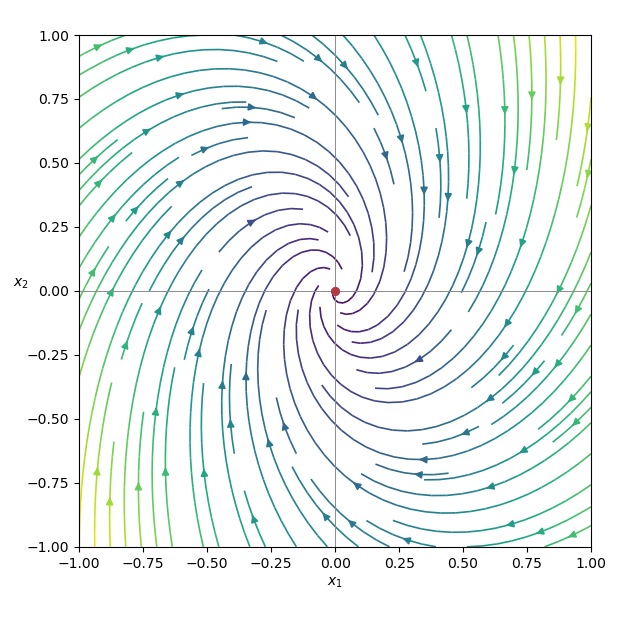
For this two-dimensional Ornstein-Uhlenbeck process, the covariance matrixsatisfiesThus the stationary covariance solves the continuous Lyapunov equationWriteSubstitution givesSolving,Therefore

For $\mathrm{Re}z>0$, integration by parts givesThe boundary term vanishes, so the Gamma function recurrence is

Given any $z\in \mathbb{C}$ that is not a nonpositive integer, choose $N$ large enough that $\mathrm{Re}(z+N)>0$ and defineThe recurrence shows that definitions from different sufficiently large $N$ agree, so this gives the unique analytic continuation from the right half-plane. It is analytic except where a denominator factor vanishes, namelyThese points are simple poles. More precisely, at $z=-n$,because one may writeand use $I(1)=1$.

Let each mass be $m$ and each spring constant be $k$, with the $x_i$ denoting longitudinal displacements from equilibrium. The Lagrangian isThe inverse coordinate transformation isSubstitution givesThus the Euler-Lagrange equations separate into a symmetric pair,and an antisymmetric pair,

The symmetric normal modes are:

For antisymmetric modes, the squared dimensionless frequencies are the eigenvalues ofnamely $2\mp \sqrt{2}$. They giveandIn the original coordinates their mode shapes are respectivelyand

The Hubble parameter is the fractional expansion rateHere $\rho$ is the homogeneous energy density, $k\in \{-1,0,1\}$ records the sign of the spatial curvature of an FLRW universe, and $R$ is the fixed curvature length scale used with the dimensionless scale factor $a(t)$.

Energy-momentum conservation in a homogeneous expanding universe gives the continuity equationDifferentiate the Friedmann equationUsing $\dot{a}/a=H$ and the continuity equation givesEliminating the curvature term with the Friedmann equation yieldsSince $\dot{H}+H^2=\ddot{a}/a$, this is the Raychaudhuri equation

Under the strong energy condition $\rho +3P\ge 0$, one has $\ddot{a}\le 0$. Thus $a(t)$ is concave, and for $t<t_0$ it lies below its tangent at the present time:The right side vanishes at $t=t_0-H_0^{-1}$. A positive scale factor therefore cannot extend regularly to that time; it must reach the Big Bang singularity at some $t_{\mathrm{BB}}\ge t_0-H_0^{-1}$. Equivalently,

Using the Pauli matrices,

In a spherical coordinate system,Since $n_x\mp i{n}_y=\sin \theta e^{\mp i\varphi }$,

The Pauli multiplication relations and $|\hat{n}|=1$ giveTherefore the possible measurement outcomes, the eigenvalues of $A$, are

The spectral projector for outcome $+1$ isFor $|1⟩=(0,1{)}^T$, the Born rule gives

The Born rule says that the probability of a projective-measurement outcome is the squared norm of the state projected onto the corresponding eigenspace. The basis vectors in the state whose second qubit is one areThey are mutually orthogonal, so

A binary block code of length $n$ is a subset $C\subseteq {\mathbb{F}}_2^n$. Its size is $M=|C|$, and its minimum Hamming distance isThus an $[n,M,d]$ code consists of $M$ binary words of length $n$ whose distinct pairs differ in at least $d$ coordinates. When $d=1$, every set of distinct words qualifies. Taking all of the binary vector space ${\mathbb{F}}_2^n$ gives $2^n$ words, and no code can contain more words than its ambient space. Hence

Form the punctured code by deleting one fixed coordinate from every codeword. Two distinct original words differ in at least $d>1$ positions, so after one deletion they still differ and cannot coalesce. The new code therefore retains size $M$, while every pairwise Hamming distance falls by at most one. It is an $[n-1,M,d^{\prime }]$ code with $d^{\prime }\ge d-1$, and hence also an $[n-1,M,d-1]$ code in the minimum-distance-at-least convention. Therefore

Iterate the puncturing inequality from part (ii) $d-1$ times and then use part (i):This is the binary Singleton bound:

Complete the square:If $M$ is even, an integer $N$ can equal $M/2$, giving the maximum $M^2/4$. If $M$ is odd, every integer $N$ is at least $1/2$ from $M/2$, giving the maximum $(M^2-1)/4$. Thus

At coordinate $j$, addition in ${\mathbb{F}}_2$ gives $x_j+y_j=1$ exactly when $x_j\ne y_j$. Therefore the number of ones in $x+y$ is exactly the number of coordinates in which the two words differ:

For column $j$, let $N_j$ of the $M$ codewords have a one. A pair contributes a one in that column exactly when one word is chosen from those $N_j$ words and the other from the remaining $M-N_j$. Hence column $j$ containsones among all pairwise sums. Part (i), summed over the $n$ columns, gives the upper boundThere are $\left(\genfrac{}{}{0ex}{}{M}{2}\right)$ rows, one for each unordered pair of codewords. By part (ii), every row has weight equal to that pair's distance, which is at least $d$. Therefore

Put $q=2d-n>0$. If $M$ is even, part (iii) givessoBecause $M$ is even,

If $M$ is odd, part (iii) instead givesCancelling $M-1$ yields $qM\le n=2d-q$, and thereforeSince $M$ is an integer, the same desired upper bound follows. Thus the binary Plotkin bound is

A register machine has finitely many natural-number registers, a finite set of labelled states, and instructions that increment a register, conditionally decrement and branch according to whether a register is zero, or halt. A program is a finite sequence of such labelled instructions, and a configuration records the current instruction together with every current register value.

Given $k$ inputs, place them in designated input registers and initialize the remaining registers to zero. The machine computes a partial computable function $f:{\mathbb{N}}^k\rightharpoonup \mathbb{N}$ when it halts with output $f(\mathbf{x})$ in the output register exactly for $\mathbf{x}\in \mathrm{dom}f$ and runs forever otherwise.

To encode a machine, encode every instruction by a natural number using effective encodings of its opcode, register number, and target labels. Encode the resulting finite sequence by a Gödel numbering, for example through iterated pairing or prime powers. Effective decoding gives an enumeration $(P_n)$ of machine programs, so the unary function computed by program code $n$ may be denoted $f_{n,1}$.

The partial recursive functions form the smallest class containing the zero function, successor function, and projection functions and closed under composition, primitive recursion, and unbounded minimization.

Fix a register machine $P$ with $k$ inputs. By the permitted result, its complete configuration after $t$ steps,is a recursive function of the inputs and time. The predicate $H(\mathbf{x},t)$ saying that this configuration is halted is therefore recursive. Its halting time is the partial recursive functionwhere unbounded minimization is undefined when no halting time exists. Extracting the output register from a configuration is recursive, sois partial recursive. Hence every partial computable function is partial recursive.

The function $g$ is not partial computable. It is defined on every input, so if a register machine with code $e$ computed it, then $f_{e,1}=g$ and in particular $f_{e,1}(e)$ would be defined. The first clause in the definition would givewhich is impossible. This is the usual diagonal argument behind the noncomputability of the diagonal halting set.

The function $h$ is also not partial computable. On every odd input it is defined, andbecause the value in the halting case is $f_{n,1}(n)+1\ge 1$. Thus a machine computing $h$ would decide diagonal halting for odd program indices simply by running $h(n)$ and testing whether its output is zero.

That restricted problem remains undecidable. By the padding lemma, an arbitrary machine can effectively be replaced by an equivalent machine having an odd code—for example by adding unreachable instructions until the chosen effective encoding has the required parity. This gives a computable reduction from unrestricted diagonal halting to diagonal halting on odd indices. A decider obtained from $h$ would therefore decide the full diagonal halting problem, a contradiction. Hence

Kilometres is an ordinal categorical variable: its five levels have a meaningful order. Treating it as an ordinary factor would use four indicator variables and hence four unrelated regression coefficients. Converting the levels to numerical scores instead imposes a single linear trend across successive mileage bands. This is more parsimonious and gives greater precision when that trend is a reasonable approximation, although it also assumes that adjacent levels are equally spaced in their effect.

The graph is a profile likelihood for the parameter $\lambda$ of a Box–Cox transformation. Its maximum is close to $\lambda =0$, and the displayed likelihood interval contains zero but excludes $\lambda =1$. Since $\lambda =0$ gives a logarithmic transformation whereas $\lambda =1$ leaves the response unchanged up to an affine transformation, the plot supports fittingas the response in model2.

Because model2 uses a logarithmic transformation, the logarithm of the payment ratio is the difference of two predicted log payments. The cars have equal Brand and Bonus values and differ by one Kilometres level, so its fitted mean is the displayed mileage regression coefficient, ${\hat{\beta }}_K=0.057132$.

For two independent future payments, the prediction interval must include both the standard error $0.032654$ of ${\hat{\beta }}_K$ and two independent residual errors. The estimated variance of the predicted log ratio is thereforeUsing the residual degrees of freedom shown in the output, a 95% prediction interval for a ratio of log-normal responses isWith $t_{284,0.975}\simeq 1.97$, this is approximately $[0.120,9.33]$. The interval is wide because it predicts the ratio of two individual future payments; an interval for the ratio of their fitted mean responses would omit the $2{\hat{\sigma }}^2$ term.

A suitable generalized linear model is a Gamma regression with logarithmic link:withThe gamma distribution is appropriate for a positive, continuous, right-skewed payment, and its variance function allows the conditional variance to grow like the square of the conditional mean instead of assuming constant variance. The logarithmic link function also guarantees positive fitted means and represents covariate effects multiplicatively, which accords with the Box–Cox transformation evidence for a logarithmic scale.