Past exam of the mathematics course of the year 2 of the natural sciences course of the University of Cambridge / 2010 / Paper 1

In Cartesian coordinates, use the Levi-Civita symbol and the Einstein summation convention to expandThe contraction of the two symbols uses the Kronecker delta, and the final step is the product rule. Thus the convective acceleration identity isPut $\mathbf{\omega }=\nabla \times \mathbf{u}$. The curl of a gradient vanishes, and the curl of a cross product identity givesSince the divergence of a curl is zero, taking the curl of the first identity yieldsTwice continuous differentiability suffices for the mixed-derivative identities used here.

Away from the axis, cylindrical coordinates put the field in the line vortex formThe only potentially nonzero component of its curl isThe other components vanish because there is no axial dependence and no radial or axial velocity. Thus the curl is zero for $\rho >0$; the field is singular on the axis, so a classical curl there is not defined.

For a spanning surface avoiding that axis, the smoothness hypotheses of Stokes theorem hold and give ${\oint }_C\mathbf{v}\cdot d\mathbf{r}=0$. If the enclosed planar region contains the axis, the singularity prevents applying that theorem directly. Excise a small disk about the origin. The resulting annulus has zero curl, so its outer circulation equals the counterclockwise circulation on the small circle:This sign assumes positive, counterclockwise orientation. Clockwise orientation gives $-\kappa$; more generally the value is $\kappa$ times the winding number about the origin. A curve through the origin is excluded because its integral is singular. In the distribution interpretation the missing vorticity is concentrated on the axis as $\kappa \delta (x)\delta (y){\mathbf{e}}_z$, explaining the nonzero circulation despite zero classical curl away from it.

Since the endpoints represent the same point of the tube, both density and diffusive flux must match. For a positive diffusion coefficient $\lambda$, the periodic boundary conditions areFor separation of variables, periodic spatial modes solve $X^{\prime \prime }+n^{2}X=0$ and have time factors $e^{-\lambda n^{2}t}$. The constant mode has no decay. The periodic diffusion on a circle solution is thereforewhere the Fourier coefficients areThe expression for $a_n$ includes $n=0$.

The specified profile is even, so $b_n=0$. Its mean follows from ${\int }_0^{\pi }(\pi -x{)}^{2}dx={\pi }^3/3$, giving $a_0=2{\pi }^2/3$. For $n\ge 1$, two integrations by parts giveConsequentlyAll nonconstant normal modes decay for $\lambda >0$, so the density becomes uniform:The conserved total amount is ${\int }_{-\pi }^{\pi }udx=2{\pi }^3/3$. The initial cusp at zero is compatible with an L2 space solution and is immediately smoothed by diffusion. At $\lambda =0$ there would be no relaxation, so positivity is needed for this long-time conclusion.

Expand the radial modified Helmholtz equation as $Ly=-y^{\prime \prime }-2y^{\prime }/x+y$. Setting $y=z/x$ gives $Ly=(-z^{\prime \prime }+z)/x$, soBoundedness at zero requires $A+B=0$, whereas boundedness at infinity requires $A=0$. The respective adapted homogeneous solutions are thereforeThe first has limit one at zero. Their Wronskian is $u{v}^{\prime }-u^{\prime }v=-x^{-2}$. Since the highest-derivative coefficient of $L$ is $-1$, the Green function must have first-derivative jump $-1$. The radial modified Helmholtz Green function on the half-line isIt is continuous at the source, and its derivative jump is $-1$, giving $L_{x}G=\delta (x-\xi )$. For fixed source it tends to $\xi e^{-\xi }$ as $x\downarrow 0$ and decays at infinity. This kernel is for the original operator and ordinary measure $d\xi$; multiplying the equation by $x^2$ would change the source normalization.

For the compact source, split the integral at $\xi =x$ when $x<R$. The needed antiderivatives areThuswhile for $x>R$ the result is $e^{-x}{x}^{-1}{\int }_0^R\xi \sinh \xi d\xi$. Simplifying givesThe continuous value at zero is $1-(R+1)e^{-R}$, and $y^{\prime }(0)=0$. Both $y$ and $y^{\prime }$ match at $R$, so no extra Dirac delta appears there. The only homogeneous solution bounded at both ends is zero, establishing uniqueness.

Split the Fourier transform integral at zero:By Fourier inversion applied to this pair, or by the residue theorem, the other transform isFor example, inversion with $\lambda =\mu$ gives $\int e^{ikx}(k^2+{\mu }^2{)}^{-1}dk=(\pi /\mu )e^{-\mu |x|}$; evenness supplies the desired sign convention.

Take the spatial Fourier transform of the Laplace equation. For $y>0$ it gives ${\hat{\psi }}_{yy}-k^2\hat{\psi }=0$. Removing the exponentially growing solution and matching the boundary givesAt $k=0$ this formula is interpreted by continuity; a single transform value does not alter the inverse integral. The previous transform pair identifiesthe Poisson kernel for the upper half-plane. The convolution theorem therefore gives the Poisson integralThis is the bounded harmonic solution for bounded decaying data, or the corresponding solution in an appropriate Fourier class. Such a growth condition matters if vertical decay is interpreted only pointwise: the nonzero harmonic function $e^{x^2-y^2}\sin (2xy)=\mathrm{Im}{e}^{(x+iy{)}^2}$ vanishes on the real axis and tends to zero for fixed $x$ as $y\to \infty$, but grows rapidly in $x$ and has no ordinary spatial Fourier transform. It can be excluded by requiring boundedness; the stated pointwise limits alone would not establish uniqueness.

For the interval data, direct integration gives the Poisson extension of interval boundary dataAs $y\downarrow 0$ it approaches $c$ for $|x|<a$, zero for $|x|>a$, and $c/2$ at $x=\pm a$. At those jump points the prescribed isolated values cannot be attained by a continuous extension; they do not affect the integral. The solution decays vertically, with $\psi \sim 2ac/(\pi y)$ for fixed $x$ and large $y$.

An eigenvalue $\lambda$ and associated eigenvector $e\ne 0$ satisfy $Ae=\lambda e$. The characteristic polynomial $\det (A-\lambda I)$ has degree equal to the positive matrix size. The fundamental theorem of algebra gives a complex root, at which $A-\lambda I$ is singular and therefore has a nontrivial kernel. Hence every nonempty square complex matrix has an eigenvector.

A nondiagonalizable example is the Jordan block $\left(\begin{array}{cc}0& 1\\ 0& 0\end{array}\right)$: its only eigenvalue is zero, and its eigenspace is one-dimensional. A Hermitian matrix satisfies $A^{†}=A$ and has an orthonormal eigenbasis by the spectral theorem. One proof finds an eigenvector, notes that its orthogonal complement is invariant, and repeats. Its eigenvalues are real becausewhere $e^{†}e>0$.

With all eigenvalues negative, $A$ is invertible. Its same complete eigenbasis givesSome powered eigenvalues can coincide, but the original eigenvectors remain a complete basis. Writing $A=U\mathrm{diag}({\lambda }_i)U^{†}$, the convergent matrix exponential series givesThus the matrix inverse from a decaying matrix exponential isThe identity printed in the original PDF is missing a minus sign. Already for the one-by-one matrix $A=(-1)$ its integral is $1$, whereas its inverse is $-1$. Equivalently, integrating $d(e^{tA})/dt=A{e}^{tA}$ gives $A{\int }_0^{\infty }{e}^{tA}dt=-I$, confirming the correction without diagonalization.

Complete the square in the quadratic form:The real invertible linear transformationsets $x_1+2x_2=y_1$, $x_2=y_2$, $\sqrt{6}{x}_3=y_3$, giving $Q_1=y_1^2+y_2^2+y_3^2$. The same transformation givesIts signature is $(2,1)$. By Sylvester's law of inertia no real invertible change of variables can turn this second form into a sum of three positive squares.

The trace of a square matrix is $\mathrm{tr}A={\sum }_i{A}_{ii}$. Expanding a product and interchanging its finite sums givesHence every commutator has trace zero. Taking the trace of $AB-BA=cI$ gives $0=cn$. Over the complex numbers, with $n\ge 1$, this forcesFor that value, choose $A=B=0$, or any commuting pair. For every nonzero $c$ the trace contradiction proves nonexistence. The finite matrix size is essential to this trace argument.

Differentiate the eigenvalue equation along the assumed smooth normalized eigenbranch:Since $A$ is real symmetric, $x^{T}A=\lambda x^T$. Multiplying the differentiated equation by $x^T$ and using $x^{T}x=1$ cancels the terms containing $x^{\prime }$:Thus the finite-dimensional Hellmann–Feynman theorem givesEquivalently, differentiating the normalization gives $2x^T{x}^{\prime }=0$ and eliminates those terms from the derivative of $\lambda =x^{T}Ax$. The proof needs the smooth eigenbranch assumed in the question; the smallest eigenvalue need not be differentiable at an arbitrary crossing without that assumption.

Evaluate the derivative along real and imaginary increments. For a holomorphic function, both give the same value:Equating real and imaginary parts yields the Cauchy-Riemann equations

Differentiate the Cauchy-Riemann equations and use equality of mixed partial derivatives, which holds because holomorphic functions are smooth:Thus both parts are harmonic functions.

The Cauchy-Riemann equations give $\nabla v=(-u_y,u_x)$. ThereforeThe gradient is normal to a regular level set, so these curves intersect orthogonally wherever their gradients are nonzero. At a stationary point, where both gradients vanish, a regular curve tangent need not exist; the algebraic identity remains valid.

The rotation $\nabla v=(-u_y,u_x)$ from the Cauchy-Riemann equations is invertible. HenceThus their stationary points coincide, including degenerate ones.

For a harmonic function, put $a=u_{xx}$ and $b=u_{xy}=u_{yx}$. Since $u_{yy}=-u_{xx}$, its Hessian matrix isA nonzero determinant is therefore negative, and the two real Hessian eigenvalues are $\pm \sqrt{a^2+b^2}$. At a stationary point the quadratic term of the Taylor expansion has both signs. Consequently every such nondegenerate stationary point is a saddle point. This is the nondegenerate stationary points of a planar harmonic function criterion. The same argument applies to $v$, whose stationary points coincide with those of $u$. A zero Hessian determinant is outside this second-order classification.

Assume the image of the domain of $f$ lies in the domain where $g$ is holomorphic. The complex chain rule givesso the composition is holomorphic, including at points where $f^{\prime }=0$. Its real part $S(x,y)=s(u(x,y),v(x,y))$ is therefore a harmonic function.

A direct verification uses the composition of harmonic conjugate pairs. The multivariable chain rule givesThe Cauchy-Riemann equations imply $|\nabla u{|}^2=|\nabla v{|}^2$; parts (i) and (ii) remove the last three terms. Since $s$ is harmonic in its own variables,

In monic form the Chebyshev differential equation has $P(x)=-x/(1-x^2)$ and $Q(x)=p^2/(1-x^2)$. Both are analytic near zero, so it is an ordinary point. At $x=1$, $(x-1)P=x/(x+1)$ and $(x-1{)}^{2}Q=-p^2(x-1)/(x+1)$ are analytic; at $x=-1$, $(x+1)P=x/(x-1)$ and $(x+1{)}^{2}Q=-p^2(x+1)/(x-1)$ are analytic. Thus both endpoints are regular singular points.

Insert $y_q={\sum }_{n\ge 0}{a}_n{x}^{n+q}$ and equate coefficients. The recurrence relation isExplicitly the factors are $(n^2-p^2)/[(n+2)(n+1)]$ for $q=0$ and $[(n+1{)}^2-p^2]/[(n+3)(n+2)]$ for $q=1$. The lowest equation for $q=1$ forces $a_1=0$. For $q=0$, one may choose $a_1=0$ to select an even solution, independent of the odd $q=1$ solution. The leading coefficient $a_0$ is free in either chosen parity branch.

For a nonterminating branch the consecutive parity-term ratio tends to $x^2$. Hence the ratio test gives convergence for $|x|<1$, and radius of convergence one. Terminating branches are polynomials with infinite radius. For $p=m\ge 0$ an integer, choose $q$ of the same parity as $m$: the recurrence stops once $n+q=m$, producing a degree-$m$ Chebyshev polynomial. Normalization at $1$ gives all nonzero coefficients through degree three:

Set $Y(\theta )=y(\cos \theta )$. Direct differentiation gives $Y^{\prime \prime }={\sin }^2\theta y^{\prime \prime }-\cos \theta y^{\prime }$, so the equation becomes $Y^{\prime \prime }+m^{2}Y=0$. For $m>0$, $Y=A\cos (m\theta )+B\sin (m\theta )$. A polynomial $y$ has finite derivative at $x=1$, and therefore $Y^{\prime }(0)=-\sin 0y^{\prime }(1)=0$, forcing $B=0$. Also $Y(0)=T_m(1)=1$, so $A=1$. For $m=0$, the transformed solution is affine in $\theta$ and the same derivative condition removes its linear term. ThusThe endpoint values follow by continuity. The finite-derivative condition is what excludes the independent nonpolynomial branch, rather than normalization alone.

For fixed endpoint values, the Euler-Lagrange equation is $f_y-d{f}_{y^{\prime }}/dx=0$. Along a stationary curve, the chain rule givesWhen $f_x=0$, the Beltrami identity therefore takes the requested sign convention

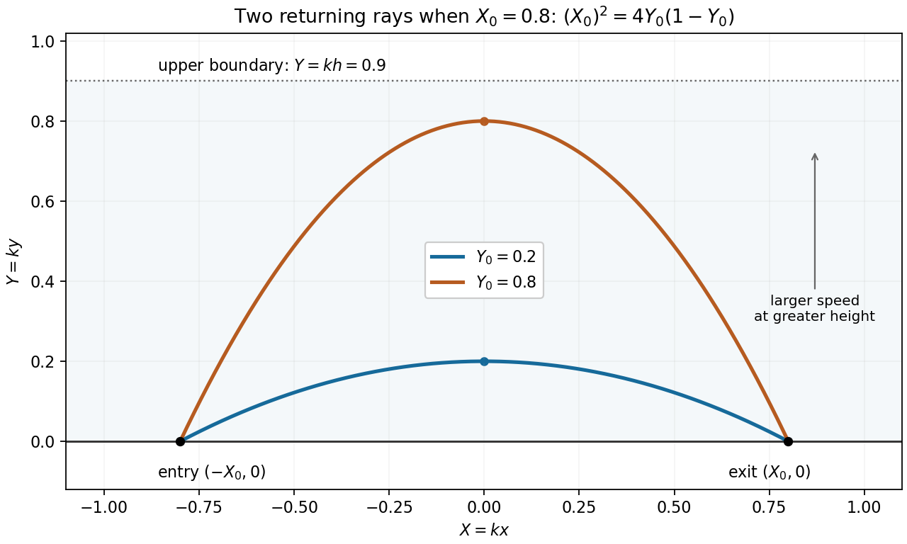
By Fermat principle, the elapsed-time integrand for the given speed is $f=c_0^{-1}\sqrt{1-ky}\sqrt{1+(y^{\prime }{)}^2}$. ThusThe constant is negative for a finite regular ray. Squaring gives $(1-ky)/(1+(y^{\prime }{)}^2)=c_0^2{A}^2$. At a maximum height $y_0$, the slope is zero, so $c_0^2{A}^2=1-k{y}_0>0$. HenceSeparate variables on either side of the turning point. Integration gives the parabolic light rays in a reciprocal-square-root speed profileThe quadratic opens downwards, with its greatest height $y_0$ at $x=x_c$. The positive index condition holds throughout the layer because $kh<1$. Vertical rays are a separate zero-horizontal-momentum case, outside the regular graph representation $y(x)$; they are not returning rays of the type considered below.

Equal endpoint heights at $x=\pm x_0$ force $x_c=0$. Setting $y(\pm x_0)=0$ givesFor nonzero separation, a real returning ray requires $k{x}_0\le 1$ and has candidate turning heightsOnly choices satisfying $0<y_0<h$ are rays wholly within the specified layer. Depending on its thickness there may be two, one, or no admissible choices; at zero discriminant the two algebraic candidates coincide. The entry and exit points at $y=0$ are interpreted as limiting boundary points of the open medium.

Use the real weighted inner product $⟨u,v{⟩}_w={\int }_a^{b}wuvdx$ and the energy bilinear form $B(u,v)={\int }_a^b(p{u}^{\prime }{v}^{\prime }+quv)dx$. Integration by parts, the endpoint conditions, and the Sturm-Liouville problem giveThus orthonormality in the stated expansion givesand hence the Rayleigh quotientThe expansion is understood for nonzero admissible functions with finite norm and energy.

For a general endpoint-preserving variation $y+\epsilon \eta$, explicitlysoThe fundamental lemma of the calculus of variations shows that stationarity is exactly the eigenvalue equation with $\lambda =\Lambda$. Conversely an eigenfunction has vanishing first variation and quotient equal to its eigenvalue. Completeness gives the same weighted-average formula for any nonzero admissible expansion, even one with zero ground-state coefficient. Since every ${\lambda }_i\ge {\lambda }_0$,This is the Rayleigh-Ritz variational principle.

For the interval problem, the normalized Dirichlet eigenfunctions and their eigenvalues, with the paper's zero-based indexing, areFor $u=x(1-x)$, direct integration gives $F={\int }_0^1(1-2x{)}^{2}dx=1/3$ and $G={\int }_0^1{x}^2(1-x{)}^{2}dx=1/30$. ThereforeThe sine expansion and Rayleigh quotient of a parabolic Dirichlet trial follow from the coefficient integralConsequently the requested expansion hasEquivalently $u=(8/{\pi }^3){\sum }_{n\ge 1,n\text{ odd}}\sin (n\pi x)/n^3$. In particular $c_1=0$: the first excited eigenfunction $\sqrt{2}\sin (2\pi x)$ is antisymmetric about $1/2$, whereas the trial function is symmetric. Since $10-{\pi }^2>0$, the final ratio is exactlyThe first nonzero correction is $c_2=1/27$, not $c_1$. Reindexing only the nonzero terms would change the meaning of the requested ratio and is not used here.