Past exam of the mathematics course of the year 2 of the natural sciences course of the University of Cambridge / 2014 / Paper 1

Work in a Cartesian coordinate system, write ${\partial }_j=\partial /\partial x_j$, and use the Einstein summation convention. For a twice continuously differentiable vector field, the contraction of two Levi-Civita symbols givesHere the Kronecker deltas select components, and equality of mixed partial derivatives gives the curl of the curl identityFor the second identity, the same contraction followed by the product rule yieldsThus the curl of a cross product isThe directional derivatives in the last two terms act on the vector field immediately to their right.

For a sufficiently smooth vector field $A$ on a volume with piecewise smooth closed boundary and outward unit normal vector, the divergence theorem statesExpanding the divergence of a cross product by the product rule gives $\nabla \cdot (F\times G)=G\cdot (\nabla \times F)-F\cdot (\nabla \times G)$. Apply the theorem to $A=F\times G$ to obtain

Use the full field in the PDF, including the exponential term missing from the transcription. Its divergence isThe exponential in the third component has zero $z$ derivative. In cylindrical coordinates, the solid has $0\le r\le 2$ and $0\le z\le 4-r^2$. Therefore the divergence theorem gives the outward fluxThe integration includes the entire closed boundary, both cap and base.

For the established time-periodic response, take a complex separated solution $v=X(x)e^{i\omega t}$ and set $u=\mathrm{Re}v$. The diffusion equation gives $X^{\prime \prime }=(i\omega /\nu )X$. For $\omega >0$, define the penetration depth $\delta =\sqrt{2\nu /\omega }$; the spatial roots are $\pm (1+i)/\delta$. Decay at infinity selectsIts real part is the solution of Stokes' second problem:The velocity amplitude decays exponentially, while the phase lags by $x/\delta$. Direct substitution verifies the diffusion equation, and the two boundary conditions follow immediately.

These data select a unique periodic response, but do not specify an arbitrary initial transient. With no initial velocity supplied, one may add any suitable solution of the homogeneous-boundary diffusion problem. The displayed solution is the usual established oscillatory flow after transients have decayed.

Separate variables as $u=X(x)T(t)$. The zero values at both plates give the Fourier sine basisExpand the initial profile using orthogonality. With $s=x/L$, its coefficients areConsequentlyOnly odd modes occur because the initial profile is symmetric about the midpoint. The coefficients are absolutely summable, so dominated convergence gives $\boxed{u(x,t)\to 0}$ uniformly as $t\to \infty$. The slowest decay rate is $\nu {\pi }^2/L^2$, associated with $j=1$.

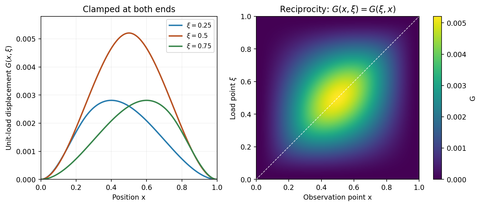
Kernel conditions. The clamped-beam Green function must obey $G(0,\xi )=G_x(0,\xi )=G(1,\xi )=G_x(1,\xi )=0$. Away from $x=\xi$, $G_{xxxx}=0$. At the load point, $G,G_x,G_{xx}$ are continuous andA jump in any lower derivative would create a derivative of the Dirac delta, rather than the single point load required by $D_x^{4}G=\delta (x-\xi )$.

Construction. A particularly simple representation isIt already enforces the left-end conditions and the correct source jump. The right-end conditions give $a+b=-(1-\xi {)}^3/6$ and $2a+3b=-(1-\xi {)}^2/2$, henceFor $x<\xi$ this is already factored; for $x>\xi$, expanding and refactoring givesThe formulas agree at the junction. The forced displacement is obtained by integrating this kernel against $f$; for continuous loads it satisfies the equation and all four end conditions. Uniqueness follows because a cubic with zero value and slope at both ends is identically zero.

Reciprocity. In terms of $x_{<}=\min (x,\xi )$ and $x_{>}=\max (x,\xi )$, the same expression isIt is visibly symmetric under interchange of $x$ and $\xi$. Thus the reciprocity of the clamped-beam Green function givesEquivalently, two integrations by parts show self-adjointness of $D_x^4$ under the clamped conditions, with bilinear form $\int u^{\prime \prime }{v}^{\prime \prime }dx$.

With the stated negative sign in the forward exponential, the inverse Fourier transform isFor example, this holds pointwise for Schwartz functions; more general square-integrable functions use the corresponding mean-square interpretation.

Differentiate under the Fourier transform integral:Hence the Fourier transform of a polynomial multiple isAbsolute integrability of the required moments justifies differentiation under the integral. The identity also extends to tempered distributions.

Let $A(k)$ be the Fourier transform of $e^{-x^2}$. Since $(e^{-x^2}{)}^{\prime }=-2x{e}^{-x^2}$, integration by parts gives $\mathcal{F}[x{e}^{-x^2}]=-(ik/2)A(k)$. Differentiation under the integral then yields $A^{\prime }(k)=-(k/2)A(k)$. The Gaussian integral supplies $A(0)=\sqrt{\pi }$, soApplying part (ii) with $n=1$ givesIt is imaginary and odd, as expected for the transform of a real odd function.

For sufficiently rapidly decaying functions, substitute the inverse Fourier transform of $g$ and interchange the integrals:The bracketed integral is the complex conjugate of $\tilde{f}(k)$. This is Parseval's identity for the chosen normalization. One may first prove it for Schwartz functions, where the interchanges are justified, and then extend it to $L^2$ by the Plancherel theorem.

Differentiating $\int e^{-a{x}^2}dx=\sqrt{\pi /a}$ with respect to $a>0$ gives $\int x^2{e}^{-a{x}^2}dx=\sqrt{\pi }/(2a^{3/2})$. ThereforeFrom part (iii), $|\tilde{f}(k){|}^2=(\pi /4)k^2{e}^{-k^2/2}$. Its frequency-side energy isin agreement with Parseval's identity.

A Hermitian matrix satisfies $H^{†}=H$, where $†$ denotes the conjugate transpose. For a nonzero eigenvector $v$ with $Hv=\lambda v$, the scalar $v^{†}Hv$ equals its own complex conjugate, andThus every Hermitian eigenvalue is real.

A unitary matrix satisfies $U^{†}U=U{U}^{†}=I$. If $Uv=\mu v$, preservation of the squared norm givesSince $v\ne 0$, $\boxed{|\mu |=1}$. These statements concern complex eigenvectors, even when the matrix entries happen to be real.

The absolutely convergent matrix exponential series givesfor Hermitian $H$. The exponents $iH$ and $-iH$ commute, so their exponentials multiply to the exponential of their sum:Hence $U$ is unitary. Alternatively, an orthonormal eigenbasis of $H$ turns the exponential eigenvalues into $e^{i{\lambda }_j}$, all on the unit circle.

Taking the adjoint of $U=M+iN$ gives $U^{†}=M-iN$. In particular, the Hermitian parts of a unitary matrix are uniquely determined:Expanding both unitary identities givesSubtracting shows $MN=NM$, and adding gives $M^2+N^2=I$. If $Mv=\mu v$, commutation implies $M(Nv)=\mu Nv$. The assumed simple spectrum makes the eigenspace one-dimensional, so $Nv=\nu v$. Thus $M,N$ have a common orthonormal eigenbasis.

On such a vector, $Uv=(\mu +i\nu )v$. If the corresponding unitary eigenvalue is $u=e^{i\theta }$, thenThe formulas for $M,N$ also show the same eigenvalue correspondence directly from $Uv=uv$ and $U^{†}v=u^{\ast }v$. Degeneracies do not prevent existence of a common basis, although the simple-spectrum assumption makes the elementary proof immediate.

The spectral theorem for real symmetric matrices supplies real eigenvalues and an orthonormal eigenbasis. Compute eigenvectors, normalize them, and within each repeated-eigenvalue eigenspace choose an orthonormal basis. Distinct eigenspaces are already orthogonal because symmetry gives $(\lambda -\mu )v^{T}w=0$ for eigenvectors with eigenvalues $\lambda ,\mu$.

Use the resulting basis vectors as columns of $O$. ThenThe order and signs of the columns can be chosen freely; rotations within a repeated-eigenvalue eigenspace are also allowed.

Use the orthogonal change of coordinatesIt preserves distances and angles and gives $x^{T}Mx=x^{\prime T}D{x}^{\prime }$. Thus the quadric surface is expressed along its principal axes asThe following three cases are the subparts of (ii) in the original PDF.

Writing the common positive eigenvalue as $\lambda$, the equation is $|x^{\prime }{|}^2=k/\lambda$. Hence it is a sphere withEvery orthonormal set of axes is a principal-axis set in this fully degenerate case.

Let ${\lambda }_1={\lambda }_2=\lambda >0$ and ${\lambda }_3=-\gamma <0$. ThenThis is a one-sheet hyperboloid of revolution around the $x_3^{\prime }$ axis. Its circular waist has radius $\sqrt{k/\lambda }$ at $x_3^{\prime }=0$, and its radius grows with $|x_3^{\prime }|$. In the original coordinates the axis is the eigenvector direction belonging to the negative eigenvalue.

The coordinate $x_1^{\prime }$ does not occur. The perpendicular cross-section isThus the surface is an elliptic cylinder extending in both directions along the zero-eigenvalue axis. Its cross-sectional semiaxes are $\sqrt{k/{\lambda }_2}$ and $\sqrt{k/{\lambda }_3}$. It becomes a circular cylinder when the two positive eigenvalues coincide.

The matrix is $M=2I-e{e}^T$, where $e=(1,1,1{)}^T$. Along $\hat{e}=e/\sqrt{3}$, its eigenvalue is $2-3=-1$. Every vector perpendicular to $e$ has eigenvalue two. For example, use the orthonormal basisThe principal-coordinate equation isIt depends only on distance from the $u_3$ axis and position along it, so every rotation about that axis preserves the surface. ThereforeThis is a one-sheet hyperboloid with waist radius $\sqrt{3/2}$. The repeated positive eigenvalue makes the two transverse principal axes nonunique.

For real-direction increments, complex differentiability gives $f^{\prime }=u_x+i{v}_x$. For imaginary-direction increments it gives $f^{\prime }=(u_y+i{v}_y)/i=v_y-i{u}_y$. Equating these expressions gives the Cauchy-Riemann equationsA holomorphic function is smooth, so mixed partial derivatives commute. Differentiating these equations givesThus both real and imaginary parts are harmonic functions:

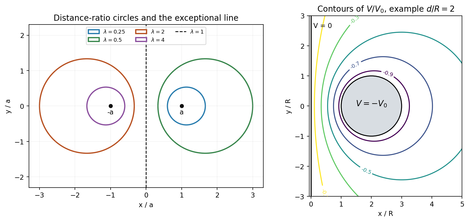
Squaring the ratio of moduli givesFor $\lambda \ne 1$, complete the square to obtain the Apollonius circleIts centre is $(a(1+{\lambda }^2)/(1-{\lambda }^2),0)$ and its radius is $2a\lambda /|1-{\lambda }^2|$. The centres are positive for $\lambda <1$ and negative for $\lambda >1$.

At the allowed exceptional value $\lambda =1$, the locus is the line $x=0$, the perpendicular bisector of the two fixed points. It is a generalized circle, but not an ordinary finite-radius circle. The point $z=-a$ is excluded from the original ratio.

For a circle in the right half-plane use $0<\lambda <1$. Its centre and radius from part (ii) satisfy $d^2-R^2=a^2$. Hence choosePut ${\tau }_0=\mathrm{arcosh}(d/R)$. Then $\sinh {\tau }_0=a/R$ andIndeed the Apollonius circle has centre $a\coth {\tau }_0=d$ and radius $a/\sinh {\tau }_0=R$. Its logarithmic modulus is therefore $-{\tau }_0$, while on $x=0$ the modulus is one. The logarithmic Dirichlet potential between a circle and a line isThe logarithmic singularity at $a$ lies inside the excluded disk, since $d-a<R$. The other singularity, at $-a$, lies outside the right half-plane. Thus the real logarithmic modulus is harmonic throughout the required region and has exactly the two specified boundary values.

Local branches of the complex logarithm justify harmonicity; its real part is globally single-valued even though the complex logarithm need not be single-valued around the excluded disk. The displayed solution is bounded and tends to zero at infinity. A boundedness or corresponding far-field condition supplies uniqueness in this unbounded domain; finite boundary values alone do not rule out unbounded additional harmonic solutions. The same geometry appears in cylinder-plane image charges.

Singular points. Normalizing the equation gives $p=2/x$ and $q=1-\ell (\ell +1)/x^2$. The only finite singular point is $x=0$, and it is regular because $xp$ and $x^{2}q$ are analytic there. At infinity put $t=1/x$ and $Y(t)=y(1/t)$; the equation becomesThe fourth-order pole makes $t=0$ an irregular singular point, so infinity is irregular.

Exponents and recurrence. Substitution of a series for a Frobenius solution gives the indicial equationWith negative-index coefficients set to zero, the coefficient equation isFor $\sigma =\ell$, it gives $a_1=0$ andFor $\sigma =-\ell -1$, it givesFor $\ell \ge 1$, $a_1=0$. At the exceptional odd index $j=2\ell +1$, the recurrence becomes $a_{2\ell -1}=0$, which is already satisfied. Thus $a_{2\ell +1}$ is free; choosing it to be zero gives an independent pure-even series times $x^{-\ell -1}$. A nonzero choice adds a multiple of the regular solution. For $\ell =0$, this freedom occurs at $j=1$ itself. This Frobenius resonance in the spherical Bessel equation is compatible, so no logarithmic term is needed despite the integer separation of exponents.

Normalized regular solution. Set $\sigma =\ell$ and $a_0=2^{\ell }\ell !/(2\ell +1)!$. The proposed even coefficientssatisfy $a_{2s}/a_{2s-2}=-1/[2s(2s+2\ell +1)]$, precisely the recurrence above. ThereforeThis is the regular Spherical Bessel function. The coefficient ratio tends to zero, so its series converges for every finite $x$; the other even-series factor also has infinite radius, although the prefactor has a pole at zero.

For $\ell =0$, the coefficients reduce to $(-1{)}^s/(2s+1)!$, givingDirectly, $x^2{j}_0^{\prime }=x\cos x-\sin x$, whose derivative is $-x\sin x$. Thus $(x^2{j}_0^{\prime }{)}^{\prime }+x^2{j}_0=0$, verifying the equation. The independent singular branch at $\ell =0$ can be chosen as $\cos x/x$.

For a variation $q\mapsto q+ϵ\eta$ with $\eta (t_0)=\eta (t_1)=0$, the first variation isThe endpoint term vanishes. Since the interior variation is arbitrary, the fundamental lemma of the calculus of variations gives the Euler-Lagrange equationAlong such a trajectory,If $L$ has no explicit time dependence, the first integral is thereforeIts negative is the equivalent Beltrami form. For the usual time-independent mechanical Lagrangian $L=T-V$ with quadratic velocity dependence, this conserved quantity is the total mechanical energy $T+V$.

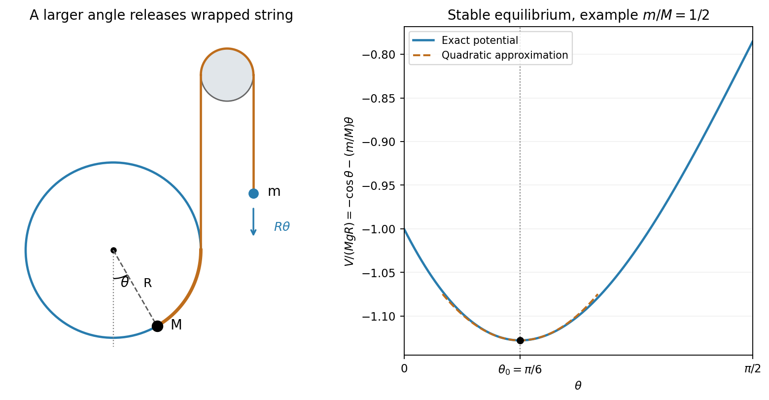
Use the angle orientation in the PDF: $M$ has coordinates $(R\sin \theta ,-R\cos \theta )$ relative to the hoop centre. The wrapped string segment has length $R(\pi /2-\theta )$. As $\theta$ increases, it releases length $R\theta$, so the suspended mass moves down by $R\theta$. Both speeds have magnitude $R|\dot{\theta }|$.

Thus the hoop with a suspended counterweight hasand $L=T-V$. The Euler-Lagrange equation givesAt equilibrium,The positive curvature $V^{\prime \prime }({\theta }_0)=MgR\cos {\theta }_0$ establishes stability. Put $\theta ={\theta }_0+\delta$ and linearize. The equilibrium force cancels, leavingHenceFor $M\gg m$, ${\theta }_0\simeq m/M$ and $\omega \to \sqrt{g/R}$, the small-oscillation frequency of a simple pendulum of length $R$. The linearization assumes an amplitude small enough to remain inside the stated angular range and a taut string throughout.

Write $N[\psi ]={\int }_a^b(p{\psi }^{\prime 2}+q{\psi }^2)dx$ and $D[\psi ]={\int }_a^{b}w{\psi }^{2}dx>0$. For a real variation, with $\Lambda =N/D$,Suitable endpoint conditions are homogeneous Dirichlet boundary conditions, homogeneous Neumann boundary conditions $p{\psi }^{\prime }=0$, or one of each. They remove the variation boundary term and the product $[p\psi {\psi }^{\prime }{]}_a^b$. Stationarity for all interior variations is equivalent toConversely, multiplication of an eigenfunction equation by $\psi$ and integration by parts gives $N=\lambda D$, hence $\boxed{\Lambda [\psi ]=\lambda }$. General Robin data require their boundary-energy contributions unless these endpoint products happen to vanish.

Use an eigenbasis orthonormal with respect to the weight: ${\int }_a^{b}w{\psi }_i^{\ast }{\psi }_{j}dx={\delta }_{ij}$. For complex coefficients use the Hermitian version of the quotient, with absolute squares. Self-adjointness givesWhen $c_0\ne 0$, dividing numerator and denominator by $|c_0{|}^2$ yieldsIf $c_0=0$, these ratios are undefined, but the unscaled formula and upper-bound conclusion remain valid. The assumptions are a problem with a self-adjoint operator bounded below and a complete eigenbasis, with the trial function in its energy-form domain. The Rayleigh-Ritz method minimizes this quotient over an admissible trial family, obtaining an upper bound on ${\lambda }_0$. Higher eigenfunctions are stationary directions and need not be unrestricted extrema.

The boundary conditions on the positive half-line, absent from the transcription, select the half-harmonic oscillator. The trial state $x{e}^{-\alpha x}$ with $\alpha >0$ satisfies both endpoints and has finite norm and energy. Integration by parts, with vanishing endpoint term, givesUsing ${\int }_0^{\infty }{x}^n{e}^{-2\alpha x}dx=n!/(2\alpha {)}^{n+1}$, the three required integrals areThus the exponential trial state for a half-harmonic oscillator gives $\Lambda (\alpha )={\alpha }^2+3/{\alpha }^2$. Its derivative vanishes at ${\alpha }^4=3$, and the arithmetic-geometric mean inequality confirms the global minimum:For comparison, the exact lowest half-line state is proportional to $x{e}^{-x^2/2}$ and has eigenvalue three. The exponential trial family gives a valid upper bound rather than an exact eigenvalue.