Source release: Oxford examination archive, member
FOI-20210708-1 - Data/a13759w1 (2).pdf. The cover dates this examination to 12 June 2017.Answer availability checked on 28 October 2026: Oxford advertises solutions for even examination years and an exceptional release for 2019; its stated policy excludes other odd years. No advertisement covering this exact paper or selected parts was found in a bounded search of official sources.[ref]
https://www.maths.ox.ac.uk/members/students/undergraduate-courses/examinations-assessments/overview-examinations. Mathematical Institute, “Past papers and model solutions”: odd-year solutions are not released, with an exception for 2019
For each interpolation node define the Lagrange cardinal polynomialAll denominators are nonzero because the interpolation nodes are distinct. Each polynomial has polynomial degree at most , and , where is the Kronecker delta. Consequently the linear combinationbelongs to the vector space of univariate polynomials and has the required values. This proves existence of the Lagrange interpolation polynomial.
For uniqueness, suppose and both work. Their difference is a polynomial of polynomial degree at most with distinct roots of a polynomial. The root bound for a polynomial forces to be the zero polynomial.
The seven supplied values follow . The quadratic polynomial belongs to and takes all seven values, so uniqueness givesThe subscript bounds the polynomial degree; it does not require polynomial degree exactly six.
The product rule applied at the interpolation node givesThus Lagrange interpolation gives, away from the interpolation nodes,Apply the same Lagrange interpolation formula to the constant polynomial one. Since its interpolant is itself,Dividing the preceding two identities proves the barycentric interpolation formulaThe denominator is exactly , so is nonzero away from the interpolation nodes. At , multiply numerator and denominator by and take the limit: their values tend to and , respectively. The removable singularity therefore has value ; in numerical evaluation return the stored value directly at an interpolation node.
A Newton-Cotes quadrature integrates a Lagrange interpolation polynomial at equally spaced quadrature nodes. For the Newton-Cotes closed quadrature, the endpoints are included: write , , and useThese quadrature weights depend on the quadrature nodes, not on the sampled function. Open Newton-Cotes quadrature uses equally spaced interior quadrature nodes instead.
For Simpson's rule, use and set , so . The Lagrange cardinal polynomials becomeIntegrating these quadratic polynomials gives , , , respectively. The change of variable contributes , soIts degree of precision of a quadrature rule is three: it integrates every quadratic polynomial by construction, and also the cubic nodal polynomial , whose integral vanishes by odd symmetry about . Any cubic polynomial differs from its quadratic polynomial interpolant by a constant multiple of this nodal polynomial.
Read the differential order literally: take quadrature nodes in and in . Applying Simpson's rule first in and then in multiplies the one-dimensional quadrature weights. With , this tensor-product quadrature isEquivalently, the nine sampled function values have the quadrature weight arraywith rows indexed by the quadrature nodes and columns by the quadrature nodes. The quadrature weights sum to the rectangle's area. If the intended coordinate assignment is instead , , exchange and in the formula. Both conventions give the same calculation on the unit square used below.
For the separable integrand, tensor-product quadrature factors into two one-dimensional applications of Simpson's rule:soThe exact double integral, evaluated by Fubini's theorem and the power rule for integration, isThe factor is always integrated exactly. All quadrature error therefore comes from applying Simpson's rule to the factor.
At , the preceding tensor-product quadrature givesBoth factors of the separable integrand are quadratic polynomials, so exactness follows directly from the construction of Simpson's rule.
At ,The factor is now a cubic polynomial. Simpson's rule still integrates it exactly because its degree of precision of a quadrature rule is three. Exactness of tensor-product quadrature depends on the polynomial degree in each variable, rather than their sum.
At ,This is an overestimate, with signed quadrature errorThe relative error is , approximately . The quartic polynomial lies beyond the degree of precision of a quadrature rule of Simpson's rule, so the exactness of the previous cases no longer applies.
Gaussian elimination uses elementary row operations to remove entries below successive pivot elements, reducing a linear system to one with an upper triangular matrix. Back substitution then solves that system. It also computes a reusable matrix factorization, so additional right-hand sides can be handled by forward substitution and back substitution without repeating the elimination.
For elimination without row exchanges, let . At step , provided the pivot element is nonzero, form the elimination multipliersand perform , applying the same operation to the right-hand side. More explicitly the resulting entries satisfy for , .
Let , where are the standard basis vectors. ThenThe matrix is a unit lower triangular matrix storing the elimination multipliers, while is an upper triangular matrix:Solving becomes followed by . If a required pivot element vanishes, an unpermuted LU decomposition can fail even for an invertible matrix. Row exchanges, typically selected by partial pivoting, instead produce with a permutation matrix ; then solve , .
Since every , the diagonal matrix is invertible. SetThe division is by the diagonal entry of row . Thus is an upper triangular matrix with diagonal entries one and .
To use symmetry without assuming the conclusion, multiply by the matrix inverse of and its transpose:The matrix is symmetric because is a symmetric matrix. It is also an upper triangular matrix, since every factor on the right is an upper triangular matrix. A symmetric upper triangular matrix is diagonal. Its diagonal is exactly , because and have diagonal entries one. Hence , givingThis is the LDL decomposition.
Take the positive square roots of the diagonal entries:The matrix is a lower triangular matrix with positive diagonal, andThis is a Cholesky decomposition. For a nonzero vector , the vector is nonzero because is invertible. ThereforeHere is the Euclidean norm. Thus is a positive-definite matrix.
For a real square matrix, a QR factorization writes with an orthogonal matrix, , and an upper triangular matrix. If is invertible, so is , andCompute and use back substitution; no matrix inverse needs to be formed.
Apply the Gram-Schmidt process to the columns . The first column has Euclidean norm two, giving and . For the second column,For the third column,This residual already has Euclidean norm one. Set and . ThusThe columns of are orthonormal, and matrix multiplication verifies .
Using precisely this QR factorization, transform the right-hand side:Back substitution in givesTherefore
A linear spline is a continuous function whose restriction to every interval is a polynomial of polynomial degree at most one. With and , linear interpolation givesIntegrating the two linear polynomials and adding the contributions givesThis is the composite trapezoidal rule applied to the nodal values, and it is exact for the linear spline itself, including nonuniform spline knots.
A cubic spline on this partition of an interval is a function that restricts to a polynomial of polynomial degree at most three on every interval . Thus its second derivative is continuous and piecewise of polynomial degree at most one: is a linear spline on the same spline knots. Its third derivative is constant on each open interval and can jump across the spline knots; its fourth derivative vanishes inside each open interval.
Put . Matching interpolation data and endpoint derivatives givesThe endpoint slope constraints make a clamped cubic spline. The decisive step in its minimum roughness property of a clamped cubic spline is the orthogonality identityProve it separately on each interval. Two applications of integration by parts, using the vanishing fourth derivative of the cubic piece, giveThe second boundary term is zero because vanishes at both endpoints of this interval. Sum over . At each interior spline knot, the two values of agree because both factors are continuous, so the contributions cancel. The remaining outer boundary terms vanish because is zero at both outer endpoints. This proves the identity.
Expanding the square now gives the stronger exact equalityThe last integral is nonnegative, proving the required inequality. It measures the excess second derivative roughness penalty of over .
The argument applies directly to twice continuously differentiable competitors. More generally it holds when is an absolutely continuous function and is square-integrable, the usual finite-energy class for this second derivative roughness penalty. Mere existence of pointwise second derivatives does not by itself guarantee that all displayed integrals exist; the variational statement is understood for admissible competitors with this regularity.
Let be a second cubic spline matching the same values and endpoint derivatives. The minimum roughness property of a clamped cubic spline applied with as the minimizing cubic spline gives , where . Applying the same argument with their roles exchanged gives . Hence equality holds, and the exact identity from part (i) yieldsThe integrand is continuous and nonnegative. If it were positive somewhere, it would have a positive integral over a small interval. It follows that everywhere. Consequently is an affine function. Its value and derivative vanish at , so it is identically zero. Thus , proving uniqueness of the clamped cubic spline with the prescribed data. Existence was assumed in the question; this argument establishes the remaining uniqueness claim.
Fix , write , , and let on this interval. The Hermite interpolation conditions give bothTwo applications of integration by parts therefore giveOn this single cubic piece, the same calculation also givesHere inside the interval, and all four endpoint values of are zero. Since , we obtain the exact identityThis is an integral inequality, with no assertion that the integrand on the left has one sign pointwise. The stronger nodal derivative conditions make the boundary terms vanish on each interval separately; part (i) only needed their cancellation after summing.
The stated Hermite interpolating polynomial exists uniquely in . Indeed, a polynomial in the kernel of a linear map of the value-and-derivative data map has a double root of a polynomial at each of distinct interpolation nodes. A nonzero such polynomial would have polynomial degree at least , which is impossible. The map is therefore an injective function and a linear map between vector spaces of the same finite dimension of a vector space, , and hence is a linear isomorphism. No higher smoothness of the original function is required to construct it.
An explicit illustration uses interpolation nodes , values , and zero derivatives at every interpolation node. The clamped cubic spline is on and its reflection on . Its Hermite interpolating polynomial is the quartic polynomial . On , , and the corresponding reflected formula holds on . Direct integration gives , , and , exactly as the energy identity predicts.
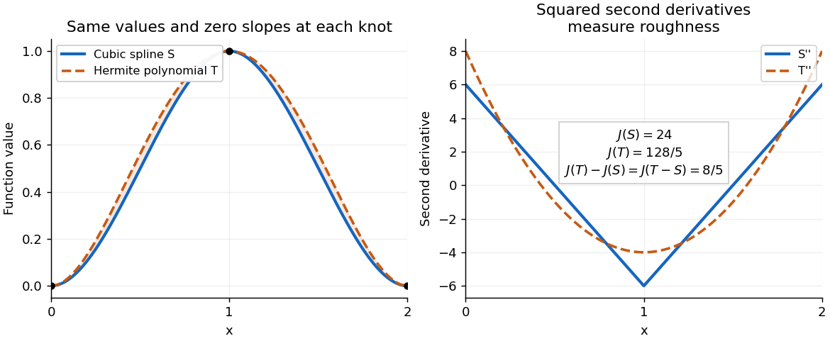
A clamped cubic spline and a Hermite interpolating polynomial with the same nodal values and derivatives: the excess second derivative roughness penalty is
. Details. 
Articles by others on the same topic
There are currently no matching articles.