Options I, Honour School of Mathematics; Friday 22 June 2007, 9.30am–12.30pm. The complete ten-page source is privately transcribed from original Part A bundle pages 10–19, supplied through the past-papers disclosure. No exact worked-answer advertisement was found in the bounded availability check.
Burnside's lemma counts the orbits of a finite group action:Identify each face with its opposite vertex. Every symmetry induces the same permutation on these two four-element sets, so a permutation with cycles fixes colorings. The rotational symmetry group is , with one identity, eight three-cycles, and three products of two disjoint transpositions. Their cycle counts are four, two and two. Thus the rotation count isAllowing reflections gives the full tetrahedral group . In addition there are six transpositions with three cycles and six four-cycles with one cycle. The count becomesEquivalently, 30 of the 141 rotational classes form 15 mirror pairs, while 111 rotational classes are their own mirror class.
The product of fixed-coloring counts is an instance of the orbit count for simultaneous colorings.
The degree is the dimension of as a vector space over . The tower theorem states that for intermediate fields in a finite extension,If the degree is prime, one factor must be one, forcing or ; no strictly intermediate field exists.
Let have 32 elements. Its prime subfield is and . Every element outside that subfield has minimal polynomial of degree five, by the tower theorem. Also every member of satisfies : nonzero elements form a group of order 31. Hence splits over , with distinct roots because its derivative is in characteristic two.
Every irreducible degree-five polynomial over divides . Indeed its quotient field has 32 elements, and its residue class of satisfies that equation. Thus every such polynomial splits into five distinct roots in . Conversely each of the 30 elements outside has one such minimal polynomial, and different minimal polynomials have disjoint root sets. Consequently the number isThere is no extra leading-coefficient factor, since every nonzero leading coefficient over is one.
Euler's theorem states that whenever , where counts the invertible residue classes. For each prime-power divisor, the same theorem gives . Since the exponent defined in the source is a multiple of every one of these exponents, raising that congruence to the corresponding integer power givesThe prime powers are pairwise coprime, so their product divides , proving the congruence modulo .
For the displayed composite integer,Thus every integer coprime to 561 satisfies . This is a Carmichael number. The source's prime-power least common multiple need not be the minimal universal exponent for all moduli; for powers of two its definition can exceed the usual Carmichael function. No minimality claim is needed here.
The monotone convergence theorem states that if measurable nonnegative functions satisfy almost everywhere on a measure space, thenallowing either side to be .
Use the nonnegative increasing truncations . They increase almost everywhere to the specified function. On each compact interval the continuous function has equal Riemann and Lebesgue integrals, so the fundamental theorem of calculus givesMonotone convergence yields . Since a nonnegative function is Lebesgue integrable exactly when its integral is finite, this function is not Lebesgue integrable.
The truncations are measurable, nonnegative, and increase almost everywhere to . As before their integrals agree with the corresponding Riemann integrals, givingMonotone convergence therefore gives the finite value . Nonnegativity makes this the integral of the absolute value as well, proving Lebesgue integrability.
A dominated differentiation theorem is the following. Suppose is measurable in and differentiable in on an open interval, is integrable for at least one parameter value, and its parameter derivative is dominated in absolute value by an integrable function independent of . Then its integral is differentiable andLocal versions require the domination only on a neighbourhood of each parameter. The proof bounds the difference quotients by the dominating function, using the fundamental theorem of calculus or the mean-value theorem, then applies dominated convergence. Apply the argument to real and imaginary parts for a complex integrand.
For fixed , is measurable and has absolute value , so is integrable. Its derivative with respect to is , whose absolute value is the assumed integrable function . HenceDominated convergence also shows this derivative is continuous, though only differentiability is required.
A sequence converges if there is such that, for every , some satisfies whenever . The limit must belong to , not merely to a larger ambient space.
A metric space is sequentially compact if every sequence in it has a subsequence converging to a point of the same space.
The sequence lies in the open interval and converges in the ambient real line to zero. Every subsequence also converges to zero, and uniqueness of limits prevents it converging to any point of the interval. Thus the interval is not sequentially compact.
For a sequence in the product, sequential compactness of supplies indices with . Apply sequential compactness of to the corresponding , extracting a further subsequence . The first coordinate still tends to . For any , both coordinate distances are eventually less than , so their sum is less than . Hence the same subsequence converges in the given product metric to . This proves the product is sequentially compact.
The subspace topology isThese sets contain the empty set and , are closed under arbitrary unions, and are closed under finite intersections because intersections distribute over the common factor . Thus they form a topology on .
For , the inverse image under inclusion is , which is open in the subspace topology by definition. The inverse-image criterion for continuity therefore proves the inclusion is continuous.
Every subspace-open set has the form for some . Continuity of makes every such inverse image open in . Hence .
If is subspace-open, thenThe right side is open in by the assumed continuity of the composition. This holds for every subspace-open set, proving is continuous into the subspace topology.
Choose and let be the identity function on . The composite is continuous by part (i). The stipulated universal implication therefore makes continuous. Its inverse image of any -open set is that set itself, so it must lie in . Thus .
The implicit function theorem applies when . After shrinking the neighbourhood, this partial derivative stays nonzero along the implicit graph. Differentiating its defining identity givesFor the specified smooth function, and , so both equal one at zero. In particular the theorem applies and . Differentiate the identity a second time:At zero, and . Therefore
Let , with at both endpoints. At an extremal the first variation is zero:Integrate the second term by parts once and the third term twice. The boundary term isThe given fundamental lemma therefore givesThis is the classical form under the usual smoothness hypotheses ensuring the displayed derivatives exist; without that extra regularity the variation first yields its distributional form.
For the concrete functional the equation is . Write , and . A general solution is . The two initial conditions give and . The final derivative condition gives , and the final value condition then gives . Thus an extremal isIt solves the differential equation, has initial value zero and initial derivative one, and at both its value and derivative vanish, using . These checks verify all four prescribed endpoint conditions.
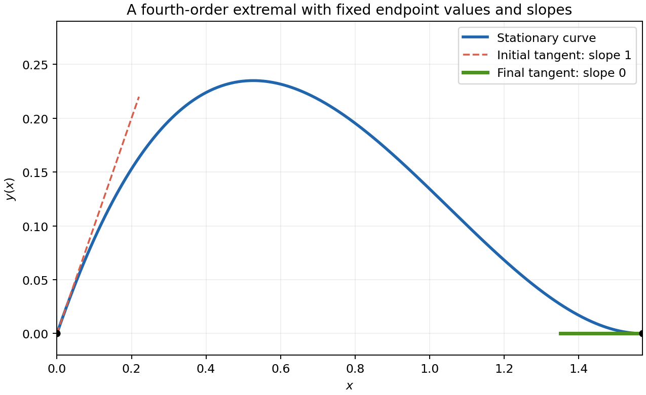
The clamped fourth-order extremal
. The computed curve satisfies both endpoint values, with initial slope one and final slope zero. Details.
Time independence conserves the energy . The two cyclic coordinates giveThese are respectively angular momentum along the symmetry axis and angular momentum along the fixed upward vertical; is the axial spin rate. For and , eliminate using . The energy becomesMultiplying and rearranging givesTo justify the double-root condition, use the effective potentialEliminating the cyclic coordinates by Routh reduction gives the remaining equation . A constant nonvertical angle therefore has and . Since , both and vanish. This argument uses the second-order equation; merely differentiating the energy identity at a stationary angle would not establish the derivative condition.
Thus steady nonvertical precession gives a common root in . The nonvertical qualification is implicit in the denominator used by the source. A top spinning exactly upright or inverted is also possible but corresponds to an endpoint , not an interior root; the unrestricted literal claim would need that exception.
The distinction is captured by the double-root criterion for steady precession of a symmetric top.
Ampère's law in magnetostatics iswith boundary and surface orientations related by the right-hand rule. Stokes' theorem gives the left side as , proving the integral law from the stated curl equation.
For a circular contour of radius about the axis, the left side is . For the enclosed current is ; for it is . ThereforeBoth expressions agree at the boundary. At the axis the field is zero, interpreted by continuity even though the angular unit vector is undefined there.
For steady flow the given equation gives . Dotting with yields , so is constant along each streamline. It can have different values on different streamlines. Dotting with also makes it constant along vortex lines where they are defined.
If the flow is additionally irrotational, and hence . Thus is one constant on each connected fluid region, the stronger global Bernoulli conclusion.
Take the curl. A gradient has zero curl, and the supplied identity, with and , givesTherefore . In planar flow and , so the stretching term vanishes. ConsequentlyVorticity is carried unchanged with each fluid particle. It need not be spatially uniform or independent of time at a fixed spatial point.
The Milne-Thomson circle theorem replaces a potential analytic inside the circle of radius by outside it, when its original singularities are outside. The circle becomes a streamline, the imposed flow at infinity is preserved, and no extra circulation is introduced.
Use the convention that positive circulation is counterclockwise, so a vortex potential is and its derivative is . With , the circle construction givesup to an additive constant and local logarithm branches. There is an image vortex of strength at and a central vortex of strength . Their zero net interior circulation is needed for the specified motion equation.
The original vortex moves with the regular velocity of the image flow, excluding its own singular velocity. ThusThe conjugation in this equation matches the printed source. Write and cancel to obtainReal and imaginary parts giveThe vortex moves uniformly on the circle determined by its initial radius, clockwise for positive in this convention.
The unit disk has area , so its joint density is . The polar-coordinate Jacobian has absolute determinant . Thereforeand is zero outside this rectangle, up to irrelevant boundary choices. Integrating givesThe joint density equals the product of the two marginal densities, so and are independent. The angle at the centre can be chosen arbitrarily since that point has probability zero.
A state is absorbing if , so once visited it is never left. Condition on the first step and use the Markov property: for , the subsequent probability of ever reaching state one is given . Hence , with .
In this chain state four is a separate absorbing state, so . The other two equations areSolving givesLet be the mean time to hit the absorbing set. From either transient state the next-step absorption probability is at least , so its tail is geometrically bounded and the expectations are finite. First-step analysis gives and . Thus and
A frequentist confidence interval is a pair of data-dependent endpoints whose random interval covers the fixed parameter with probability at least under every allowed parameter value. In repeated uses of the same sampling procedure, at least the advertised fraction of intervals cover the true value. It is not a posterior probability assigned to the parameter after observing the data.
For a sample of size from a Poisson law with mean , the sum is Poisson with mean . At observed , define the lower and upper limits byAt set and use the same upper equation. This inverts the two exact one-sided tail tests. Discreteness means the resulting central interval is generally conservative: its coverage is at least the nominal value, not identically equal to it.
Here one observes a four-year total of 39, so the lower endpoint satisfies and the upper satisfies . Selecting the corresponding entries supplied in the source givesThis interval concerns the expected four-year total, not an annual rate. The other two supplied numbers correspond to the wrong inclusive tail for one of these endpoints.
The power of a test at a parameter value is its probability of rejecting the null there. Its size is the supremum of this probability over the null parameter set. The Neyman-Pearson lemma states that for simple null and alternative densities , a test rejecting where , accepting where , and randomizing as needed on equality to attain size , has greatest power among tests of size at most .
The specified function is nonnegative. Its integral isFor independent observations write . The likelihood ratio of the smaller alternative parameter to the null isIt is strictly increasing in . Thus the most powerful level- test rejects forThe continuous distribution permits this size without randomization for . Its threshold depends only on the null and the desired size, not on which was chosen. The same test is therefore uniformly most powerful against the entire one-sided alternative .
A Givens rotation equals the identity except in coordinates , where its block can be taken asThe two block columns are orthonormal because ; other coordinates are unchanged, so the full matrix is orthogonal. If , take , and . The transformed pair is . If both entries are zero, the identity already suffices.
For the specified vector one possible matrix isIts rows are orthonormal. It is not unique: premultiply by any orthogonal transformation fixing the second coordinate axis pointwise. This rotates or reflects the other two output coordinates without changing the required image. Equivalently its second row must be , but any orthonormal completion of that row works.
Richardson extrapolation cancels a leading discretization error by combining two mesh sizes. If with , thenUse a uniform grid , , with even . The composite trapezium rule isThe composite Simpson rule, formed by integrating a quadratic interpolant on each pair of successive panels, isAssume an even-power trapezium error expansion ; continuous fourth derivative is a standard sufficient smoothness hypothesis. The coarse grid has step , so one extrapolation step is . Its endpoint coefficients are , its odd-index coefficients are , and its interior even-index coefficients are . ThereforeThe algebraic identity between the two rules holds for any sampled values; the smoothness and error assumptions are used to infer the improved accuracy.
Articles by others on the same topic
There are currently no matching articles.