The Holstein–Primakoff transformation converts a spin algebra into bosonic operators while retaining the finite physical spin Hilbert space. With , writeThe Holstein–Primakoff occupation constraint is . Acting on , the raising matrix element is and the lowering element is . Their squared difference is , reproducing . Operator ordering inside the square roots is essential. For low boson occupation relative to , expand them to obtain and . Keeping quadratic terms gives the linear spin-wave approximation; higher terms describe magnon interactions. Large helps control the expansion, but a low-dimensional infrared divergence can invalidate it even at large finite .
For the ferromagnet choose , , with unit lattice spacing and . Expand around the all-up state. A longitudinal bond contributes , and the transverse exchange contributes . After a Fourier transform,These are ferromagnetic magnons. The polarized vacuum is an exact ground state of the full ferromagnetic Hamiltonian: every bond is in its maximum total-spin sector, minimizing that bond energy. It therefore has no quantum zero-point reduction of its magnetization. The one-magnon dispersion is also exact, although interacting many-magnon states need not be free bosons. Rotating the polarization generates the maximum-total-spin ground-state multiplet. Selecting a definite direction in a thermodynamic symmetry-breaking description breaks to ; the two transverse spin components form a canonical pair, producing a single quadratic type-B Goldstone boson. A small aligning field gaps it by the Zeeman energy.
At nonzero temperature the one-dimensional ferromagnet is different: its thermal magnon number contains , with infrared behaviour . The divergent magnetization reduction signals the absence of finite-temperature long-range order in an infinite short-range isotropic chain, consistent with the Mermin-Wagner theorem. It does not disallow the polarized zero-temperature ground states just constructed.[ref]
For the antiferromagnet use , still , on an even bipartite chain. The classical reference state alternates up and down. Rotate one sublattice through so that both local quantization axes point along their reference spins. In unrotated physical components, to leading order , , and . Choosing Fourier phases using the actual site positions givesThe reduced Brillouin zone has momenta and length . The pair creation and annihilation terms express the fact that an antiparallel reference product state is not an eigenstate. A bosonic Bogoliubov transformation with , , diagonalizes each two-mode block. With the sign convention and , the result isThus the harmonic antiferromagnetic modes have linear, rather than quadratic, long-wave dispersion. In an unfolded Brillouin-zone description the same result is represented by zeros at both zero and the antiferromagnetic wavevector; these are not extra independent degrees of freedom beyond the two-sublattice accounting.
The Bogoliubov vacuum has no or excitations but contains original spin bosons, with . Its staggered magnetization is . This quantum depletion of Néel order diverges logarithmically at small in one dimension. Linear spin-wave theory therefore does not establish a stable ordered antiferromagnetic ground state for this chain. Its nominal gapless dispersion is a result of expanding around an invalid ordered reference, not a general proof of the exact excitation spectrum. For the nearest-neighbour isotropic chain, integer-spin systems have a Haldane gap, whereas half-integer-spin systems are gapless; the spin-one-half chain in particular has fractional spin excitations rather than a simple dilute gas of ordered-state magnons. This distinction requires physics beyond the harmonic expansion, including the topological term in the continuum theory.[ref]
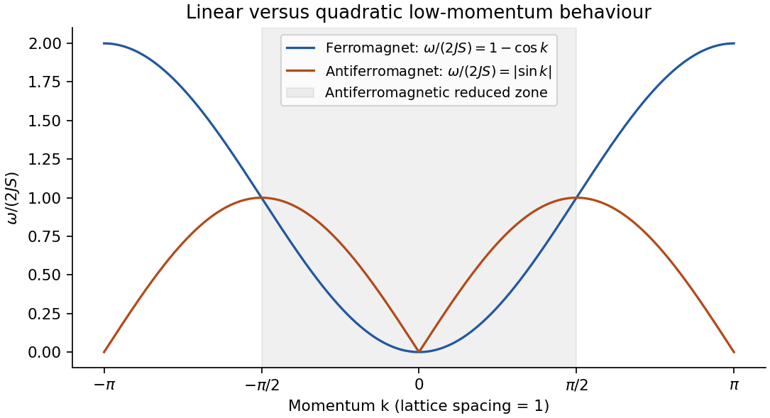
Original harmonic chain dispersions; the antiferromagnetic curve is a spin-wave approximation, not the exact spectrum for every spin
. Details. 
For one coordinate with Hamiltonian , the propagator is , where . Divide into intervals , use the Trotter product formula to separate kinetic and potential evolution, and insert complete position and momentum bases at each slice. The momentum integral is Gaussian:Multiplying the short-time kernels gives the time-sliced configuration-space path integral,with , . Continuum notation abbreviates this limit as , where . The measure includes the displayed normalization; it is not an unweighted count of paths. A small damping or analytic-continuation prescription defines the oscillatory integrals. The paths contribute complex amplitudes, so alternative histories interfere before probabilities are calculated. This is the central difference from a classical statistical mixture of trajectories.[ref]
Space-Time Approach to Non-Relativistic Quantum Mechanics by Richard Feynman. pp.367–374, action phases and construction of the propagator
When actions vary rapidly relative to , stationary phase selects classical paths. Put , with zero at the endpoints. Vanishing first variation gives . The quadratic term isThe resulting Gaussian fluctuation determinant is the semiclassical propagator prefactor. In one dimension, away from caustics,The branch convention makes for a direct free-particle path before any caustic. The Maslov index tracks the phase changes as fluctuations pass through a focal singularity. In several dimensions replace the endpoint derivative by the Van Vleck determinant. The approximation sums all relevant classical paths; real-time action need only be stationary, not a minimum. It fails in this simple form at a caustic or coalescing saddles, where a uniform approximation is needed. Quadratic actions have no higher fluctuation terms, making their Gaussian evaluation exact. For example gives the exact free-particle kernel . Tunnelling involves classically forbidden regions and can be described by imaginary-time saddles rather than real classical trajectories.
Quantum statistical mechanics follows by Wick rotation . The imaginary-time evolution operator is , with Euclidean actionTaking a thermal trace identifies and integrates the endpoint positions:This thermal trace as a closed Euclidean path integral explains the periodic imaginary-time direction. A density-matrix element instead retains open endpoints. For many identical particles the trace also sums over endpoint permutations, with a plus sign for bosons and permutation parity for fermions. In coherent-state language this becomes periodic bosonic fields and antiperiodic Grassmann fields, with corresponding Matsubara frequencies.
The Euclidean weight resembles a classical Boltzmann weight. A time-sliced local quantum field in spatial dimensions becomes a classical-looking field model in dimensions, with anisotropic couplings and extra extent . Thus zero-temperature quantum criticality can be treated using an infinitely extended imaginary-time direction, while nonzero temperature imposes a finite thickness. The dynamical scaling of time need not equal the spatial scaling: the dynamical critical exponent specifies their relationship. This quantum-to-classical imaginary-time mapping requires qualification when weights have signs or imaginary terms; such a functional integral is not automatically an ordinary positive classical probability distribution. Even with a positive weight, the mapping concerns equilibrium statistics, not literal dissipative real-time trajectories. For a free particle the Euclidean kernel is a diffusion kernel with diffusion coefficient , illustrating the mathematical correspondence.
The classical high-temperature limit is a further approximation, rather than simply another name for imaginary time. If quantum level spacings and exchange effects are negligible, a one-particle partition function in dimensions becomesFor indistinguishable particles there is a factor in the dilute classical gas, and exchange is negligible when the number density times the thermal de Broglie wavelength to power is small. For a harmonic oscillator, the exact quantum result tends to as , recovering the classical phase-space integral. stationary phase explains classical mechanics; the short imaginary-time, weak-exchange limit explains classical statistical mechanics. These are related but distinct limits of the same quantum formulation.
Consider a conventional spin-singlet, weak-coupling, three-dimensional superconductor. Set in the microscopic action and restore electromagnetic units below. An attraction in an energy shell about the Fermi surface gives a Grassmann actionThe attractive sign permits pairing even when the single-particle Fermi gas is otherwise stable. A complex Hubbard–Stratonovich transformation introduces a pair field proportional at the saddle to . The action is then quadratic in fermions. Integrating them out gives the BCS pairing-field effective actionHere the trace uses one independent Nambu spinor pairing block; a fully doubled particle-hole representation instead carries its corresponding one-half factor. At a uniform saddle the Bogoliubov--de Gennes Hamiltonian can be written asThe negative branch describes the paired vacuum; excitations are Bogoliubov quasiparticles mixing particles and holes. Extremizing the effective action givesThe physical cutoff or a renormalized interaction is part of the microscopic model; an unregulated contact integral must not be used indiscriminately. With constant density of states per spin and shell half-width , the zero-temperature weak-coupling solution is . The exponentially small scale follows from the logarithmic pairing susceptibility of states near the Fermi surface. For this ideal weak-coupling model, . The microscopic theory relates the gap, pairing and thermodynamic transition.[ref]
Theory of Superconductivity by John Bardeen and others. pp.1175–1177 and the energy-gap and finite-temperature developments
Close to a continuous transition, for fields varying slowly compared with microscopic scales, expand the effective action in powers and gradients of . Its static part is the Ginzburg-Landau theory of superconductivity:The normalization of fixes the coefficients; here changes sign at . The uniform minimum has for , condensation free-energy density , and characteristic coherence-length scale . Above the transition the minimum is at zero. The quartic stabilization and gradient cost are precisely the ingredients of Landau theory for a complex order parameter. This controlled near-transition expansion supplies a bridge between microscopic BCS theory and macroscopic magnetic response; its coefficients and validity depend on the material and fluctuation regime.[ref]
Microscopic Derivation of the Ginzburg-Landau Equations in the Theory of Superconductivity by Lev Gor'kov. pp.1364–1367, microscopic expansion near the transition
Write . The radial fluctuation has positive local restoring curvature, whereas the phase has no local potential in a neutral theory with global symmetry. Freezing the amplitude givesThe neutral case supports a gapless collective phase mode. In the charged case the electromagnetic field couples to this phase rigidity. Under and , the displayed combination is invariant. Locally choosing a gauge with constant phase leaves a quadratic term in . Varying the free energy gives the transverse London current and magnetic screening scale,Combining this relation with static Maxwell equations gives exponential field penetration, the Meissner effect. Single-valuedness of the pair field around a loop with negligible current gives flux in units . These are gauge-invariant physical consequences of the condensate stiffness.
For the dynamics, the neutral phase and density mode is reorganized by the Coulomb interaction and the dynamical electromagnetic field. In a bulk three-dimensional system the long-wave longitudinal mode has a plasma gap, rather than remaining the neutral sound mode. This is the Anderson-Higgs mechanism in a superconductor: a phase coordinate becomes part of the electromagnetic collective response instead of surviving as an independent massless physical particle. Local gauge transformations are redundancies of the description, so a literal breaking of a local redundancy is not an observable. Phase coherence, current response and magnetic screening provide the physical statements.[ref]
Plasmons, Gauge Invariance, and Mass by Philip Warren Anderson. pp.439–442, plasma oscillations and the charged versus neutral matter spectrum
A static Landau functional alone cannot determine that full dynamical spectrum. A two-dimensional film, for example, need not have the same long-wave plasma dispersion as a bulk charged system. Nor does a positive radial curvature automatically guarantee a sharp Higgs amplitude resonance: coupling to quasiparticles and other modes can damp it. The chosen mean-field phase is also a thermodynamic symmetry-breaking description; an isolated finite system can be formulated with definite particle number. The microscopic pairing saddle, the near-transition Landau expansion and the electromagnetic Anderson-Higgs response describe successive scales of the same superconducting state, with distinct assumptions at each step.
Articles by others on the same topic
There are currently no matching articles.