Past exam of the short options paper shared by Prelims and Parts A and B of the physics course of the University of Oxford / 2018 / S2 (Astrophysics: from planets to the cosmos)

The distance modulus at $100\mathrm{pc}$ is five magnitudes. Thus the two approximate main-sequence endpoints read from the original figure, $m_V\simeq 0,20$, correspond to $M_V\simeq -5,15$. With the given solar reference,Use the figure's approximate endpoint effective temperatures $25,000$ K and $2500$ K. If $V$-band luminosity is used as a rough bolometric proxy, the Stefan–Boltzmann law givesTaking $T_{\odot }\simeq 5800$ K givesThese are schematic estimates, not precision radii. The diagram supplies $V$ magnitudes rather than bolometric luminosities, and hot and cool endpoints need different bolometric corrections. The exact range cannot be recovered without those corrections; the quoted values state the intended approximation explicitly.

Integrating $dP/dr=-G{M}_r\rho /r^2$ in order of magnitude, with $\rho \sim M_{\ast }/R_{\ast }^3$, givesThe ideal gas law independently gives $P_c\sim M_{\ast }{k}_B{T}_c/(\mu m_H{R}_{\ast }^3)$. Equating the two estimates yieldsFor similar composition and an approximately fixed hydrogen-burning central temperature, $R_{\ast }\propto M_{\ast }$. Calibrating this rough relation on the Sun and using part a gives a nominal mass range of about $0.05$ to $5M_{\odot }$.

The endpoint luminosity ratio is $10^8$, whereas the inferred mass ratio is about $10^2$, giving $L\propto M^4$ across that range. The exponent is therefore consistent at this schematic level. The solar normalization and individual endpoint masses are much less reliable: using the luminosity relation itself gives approximately $0.1$ to $10M_{\odot }$. Central temperatures are not truly constant, low-mass stellar structure differs, and the uncorrected $V$ luminosities in the diagram are not bolometric. These limitations prevent treating the rough radius-based masses as a contradictory precision measurement.

If radiation dominates the central pressure, equate $P_c\sim G{M}_{\ast }^2/R_{\ast }^4$ to $a{T}_c^4/3$. This givesAt roughly fixed burning temperature, the corresponding mass-radius scaling is $R_{\ast }\propto M_{\ast }^{1/2}$, rather than the gas-pressure estimate $R_{\ast }\propto M_{\ast }$. Radiation pressure alone does not determine a unique radius at a specified mass: a thermal or nuclear-burning condition is still needed to specify $T_c$. The relation is a homology estimate, not a universal exact law for all massive stars.

The numbered features in the original colour-magnitude diagram have the following interpretation.

Continuous star formation explains the coexistence of newly formed massive main-sequence stars with evolved low-mass remnants; interpreting a single sharp turnoff as the age of a coeval cluster would be inappropriate here.

At this small redshift, $D\simeq cz/H_0\simeq 20.0$ Mpc. The outer angular radius gives $R_{\mathrm{out}}\simeq D\theta \simeq 21.3$ kpc. Approximating the dynamical mass by a spherical equivalent,The supplied Tully-Fisher relation gives $M_V\simeq -22.49$, and hence $L_V\simeq 9.9\times 10^{10}{L}_{V,\odot }$. Treating the population as solar-like gives the estimate ${{\rm Y}}_V\simeq 1M_{\odot }/L_{V,\odot }$, soThe dynamical estimate exceeds that by about a factor of five; a massive extended dark-matter component is the natural interpretation. Solar-like spectra do not exactly fix the population mass-to-light ratio, and a disk is not spherical, but order-unity corrections do not remove this large outer mass excess under the stated estimate.

The effective radius is one tenth of the optical outer radius: $R_e\simeq 2.13$ kpc. A flat rotation speed then gives $M_{\mathrm{dyn}}(<R_e)\simeq 4.9\times 10^{10}{M}_{\odot }$. Half the luminosity, with the same mass-to-light ratio, implies $M_{\mathrm{luminous}}(<R_e)\simeq 4.9\times 10^{10}{M}_{\odot }$.The concentration of light into a small fraction of the optical radius suggests a high-surface-brightness, centrally concentrated disk galaxy, plausibly an early-type spiral or lenticular with a substantial bulge. The kinematic and photometric data do not uniquely distinguish those morphologies. Disk geometry, an unknown inclination correction, or a varying stellar mass-to-light ratio would alter the exact numerical inner comparison.

Using the same luminosity estimate, the distance modulus is $12.5-(-22.49)=34.99$, implying $D\simeq 99.4$ Mpc. Pure Hubble expansion at that distance predicts about $7450\mathrm{km}{\mathrm{s}}^{-1}$. The measured velocity therefore impliesIts line-of-sight peculiar velocity is toward us, of the order expected for orbital motions in a rich galaxy cluster. A galaxy falling toward a cluster centre from its far side could have this sign. Its actual front/back location or three-dimensional orbit is not determined without the cluster's mean velocity, distance and projected position. Tully-Fisher scatter and the assumption of identical luminosities also limit that inference.

Let $I$ denote a characteristic surface brightness and ${\rm Y}=M/L$ the relevant dynamical mass-to-light ratio. With comparable profiles, $L\propto I{R}^2$ and $M\propto V^{2}R/G$. Eliminating $R$ givesIf both $I$ and ${\rm Y}$ are independent of speed, converting luminosity to magnitude gives $M_V=\text{constant}-10{\log }_{10}V$. The empirical coefficient $-8$ instead means $L\propto V^{3.2}$, and thereforeFor constant surface brightness this requires ${\rm Y}\propto V^{0.4}$; for constant mass-to-light ratio it requires $I\propto V^{0.8}$. A mixture of these changes, including varying stellar populations or dark-matter fractions, can give the same observed slope. The simple derivation assumes comparable characteristic radii and structural coefficients.

The curvature constant specifies the intrinsic spatial curvature of homogeneous constant-time slices. Positive curvature has spherical geometry, zero curvature Euclidean geometry, and negative curvature hyperbolic geometry. A conventional coordinate normalization uses $k=+1,0,-1$, with the scale factor carrying the curvature radius; rescaling that factor changes the numerical magnitude assigned to a dimensional curvature coefficient.

The sign alone does not determine the future expansion once a cosmological constant is admitted. Nor does negative or zero local curvature by itself determine the global topology: quotient spaces can share the same local curvature.

For conserved nonrelativistic matter, ${\rho }_M={\rho }_{M0}{a}^{-3}$, where $a=R/R_0$ and $a_0=1$. Substitution into the Friedmann equation giveswithThe source writes the dimensionless normalized factor as $R$ in its final expression; this is equivalent to setting $R_0=1$ consistently in the curvature coefficient. Evaluating today gives ${\Omega }_M+{\Omega }_k+{\Omega }_{\Lambda }=1$. Here the printed $\Lambda$ already has dimensions of inverse time squared. If the cosmological constant is instead defined geometrically with inverse-length-squared units, replace this $\Lambda$ by ${\Lambda }_{\mathrm{geom}}{c}^2$.

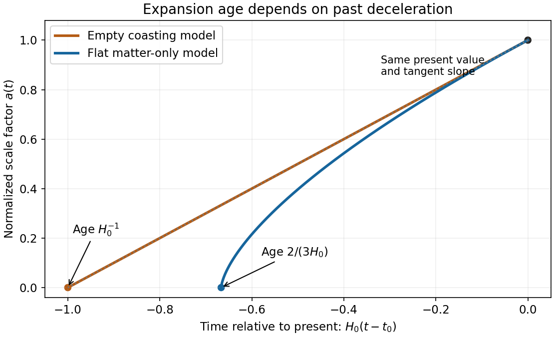
With zero curvature and no cosmological constant, the present normalization requires ${\Omega }_M=1$. Thus $\dot{a}=H_0{a}^{-1/2}$, and choosing the big bang as $t=0$ givesFor an empty expanding model, ${\Omega }_k=1$ and the curvature must be negative. The equation becomes $\dot{a}=H_0$, givingThe latter is the Milne slicing of flat spacetime; its zero-scale-factor origin is not a matter-density curvature singularity. In the matter model, gravity decelerates expansion, so the earlier slope was greater than the present slope and the same present size was reached in less time. With the stipulated $H_0$, the two model ages are approximately $8.69$ and $13.0$ Gyr.

Adiabatic photon redshifting gives $T\propto a^{-1}$. Using the stipulated temperatures,In the flat dust approximation of part c, $t=t_0{a}^{3/2}$, so $t_{\mathrm{rec}}\simeq (2/3H_0)1000^{-3/2}\simeq 2.75\times 10^5$ years. This approximation omits the significant radiation contribution near the actual recombination epoch.

The elementary travel-distance estimate is $c{t}_{\mathrm{rec}}\simeq 8.4\times 10^4$ pc, whose corresponding comoving scale today is about $84$ Mpc. In an expanding universe, however, that is not the exact proper particle-horizon radius. Integrating the null geodesic givesfor dust. Thus the proper horizon at this epoch is about $0.25$ Mpc and its present comoving size about $250$ Mpc. The factor three accounts for expansion during light propagation. These scales describe the limited causal domain in the simple decelerating model. The near-uniform CMB temperature across much more widely separated last-scattering regions motivates the horizon problem; the question's rough $ct$ estimate and the exact dust horizon should not be conflated.