Original examination: Functional programming, data structures and algorithms, procedural programming, and digital hardware examination paper by the University of Oxford (2003).
Use pattern matching to separate the empty list from a head and tail. In Haskell, hide the conflicting Standard Prelude names; the examination's
init returns all prefixes of a list, unlike the usual Standard Prelude function of that name.import Prelude hiding (map, length, init, tails, foldr, compare)
map :: (a -> b) -> [a] -> [b]
map f [] = []
map f (x:xs) = f x : map f xs
length :: Num n => [a] -> n
length [] = 0
length (_:xs) = 1 + length xs
copy :: (Eq n, Num n) => n -> a -> [a]
copy 0 xs = []
copy n xs = xs : copy (n-1) xs
combine :: [[a]] -> [[a]] -> [[a]]
combine [] _ = []
combine _ [] = []
combine (xs:xss) (ys:yss) = (xs ++ ys) : combine xss yss
init :: [a] -> [[a]]
init [] = [[]]
init (x:xs) = [] : map (x:) (init xs)
tails :: [a] -> [[a]]
tails [] = [[]]
tails (x:xs) = (x:xs) : tails xsThe map function preserves the input list shape while transforming each entry.
length counts the cons cells. copy repeats the whole value xs, so for the specified use its second argument is a list and the result is a list of lists. Its inferred type is more general: the repeated value can have any data type. If one restricts the interface to lists, the corresponding type is (Eq n, Num n) => n -> [a] -> [[a]]. The numeric argument has the precondition that it is a nonnegative integer; the most general inferred numeric constraints do not guarantee termination on arbitrary values of their instances. An explicitly integral interface may instead use Integral n => n -> [a] -> [[a]].combine performs list concatenation head by head and stops as soon as either outer list ends. For init, every nonempty prefix of a list starts with x and continues with a prefix of a list from xs; prepending [] supplies the shortest prefix of a list. For tails, the longest suffix of a list is the whole input, followed by all suffixes of a list of its tail. For example, init [1,2] = [[],[1],[1,2]] and tails [1,2] = [[1,2],[2],[]]. Thus both include the empty list, andUse structural induction on the first finite outer list
xss, with the assertion quantified over every finite yss. For xss = [], both sides are []. For the nonempty case of structural induction, write xss = xs:xss'. If yss = [], both sides again truncate to []. Otherwise write yss = ys:yss'. Expanding the definitions givesThe second equality uses the defining equation for list concatenation and the induction hypothesis for the smaller outer list xss'. The argument covers unequal outer lengths because the empty second list was handled explicitly. HenceFor finite lists, Cartesian lifting of a binary operation to lists preserves associativity. Both associations enumerate triples in the same order: the entry from
xs changes slowest, then the entry from ys, then the entry from zs changes fastest. The results are respectivelyandAssociativity makes corresponding entries equal; their order and multiplicity already agree. Empty lists make both sides empty. ThereforeCommutativity of the element binary operation does not remove the ordering of a list comprehension. For ordinary addition, take
xs = [1,2] and ys = [10,20]. ThenThe middle entries occur in opposite orders. HenceIdempotence concerns applying an operation to the same whole value. It says more than saying that the equal-entry pairs are unchanged. Choose the idempotent binary operation
min. ThenMore generally, a finite list of length paired with itself produces entries, so length alone contradicts idempotence when . ThereforeA right fold replaces the empty list by a seed and each cons by an application of the combining function:
foldr :: (a -> b -> b) -> b -> [a] -> b
foldr op e [] = e
foldr op e (x:xs) = op x (foldr op e xs)Each entry contributes a choice between omission and inclusion. Use list concatenation as , so that Cartesian lifting of a binary operation to lists joins every choice from an earlier position to every choice from later positions:
crossAppend :: [[a]] -> [[a]] -> [[a]]
crossAppend xss yss = [xs ++ ys | xs <- xss, ys <- yss]

f :: a -> [[a]]
f x = [[],[x]]

subs :: [a] -> [[a]]
subs xs = foldr crossAppend [[]] (map f xs)
The seed is
[[]], because the empty list has one subsequence, namely [], and concatenating the empty list changes nothing. If rest lists the subsequences of the tail, crossAppend [[],[x]] rest lists all omissions of x first and all inclusions second. For [a,b,c], the last position changes fastest, producing the specified order [], [c], [b], [b,c], [a], [a,c], [a,b], [a,b,c]. Repeated input values can give equal subsequences at distinct choices of positions; those repetitions are retained. ThusA string data type suffices for a name, an algebraic data type for the recorded sex, and a triple of integers for a date. Use a constructor for
Person so that selectors are unambiguous in Haskell:type Name = String
data Sex = Female | Male deriving (Eq, Show)
data Date = Date { day :: Int, month :: Int, year :: Int }
deriving (Eq, Show)
data Person = Person { name :: Name, sex :: Sex, born :: Date }
deriving (Eq, Show)
type BirthCertificate = (Person, Person, Person)
type Database = [BirthCertificate]Dates have the precondition that their fields form a valid calendar date. This simple database representation assumes the triple of identifying fields distinguishes the recorded individuals; a production database would normally add a stable identifier to distinguish namesakes. The two constructors for
Sex model the two recorded values used by this exercise. In mathematical notation,Extract the two recorded parents from every matching certificate, and use duplicate removal so that repeated certificates do not repeat an individual. This helper is shared by the remaining Haskell definitions:
unique :: Eq a => [a] -> [a]
unique [] = []
unique (x:xs) = x : unique [y | y <- xs, y /= x]

parents :: Database -> Person -> [Person]
parents db p = unique [q | (baby,mother,father) <- db,
                          baby == p, q <- [mother,father]]
A person need not have a certificate of their own to appear in the output: a parental field is already evidence of the relationship. The resulting list preserves first occurrence order, with mother before father in each certificate. Its set of entries is
children :: Database -> Person -> [Person]
children db p = unique [baby | (baby,mother,father) <- db,
                              mother == p || father == p]
Duplicate removal handles repeated certificates and children recorded in more than one matching row. ThusThe displayed set describes membership; the implementation returns its entries as a list in first certificate order.
Treat brothers as male individuals sharing at least one recorded parent, including half-brothers. Derive a sibling helper and then select the recorded sex:
siblings :: Database -> Person -> [Person]
siblings db p = unique [q | parent <- parents db p,
                           q <- children db parent, q /= p]

brothers :: Database -> Person -> [Person]
brothers db p = [q | q <- siblings db p, sex q == Male]
The exclusion
q /= p prevents a male individual from being his own brother. Duplicate removal is needed because a full brother can be found through both parents. The membership condition isIf the intended convention is full brothers only, replace the shared-parent condition by a common mother and a common father in the recorded certificates. The definition above states the convention explicitly rather than silently discarding half-brothers.Use first cousins: the children of the siblings of a recorded parent. This includes cousins through a parent's half-sibling under the convention above. In Haskell:
cousins :: Database -> Person -> [Person]
cousins db p = unique [q | parent <- parents db p,
                          auntOrUncle <- siblings db parent,
                          q <- children db auntOrUncle, q /= p]
Selecting siblings of parents avoids the mistake of returning all people with a common grandparent, which would also return ordinary siblings. The explicit exclusion of
p is harmless on an ordinary consistent pedigree and prevents a self-result in unusual records. Multiple relationship paths give just one output entry after duplicate removal. ThusAn individual can have any number of children, so use a rose tree, with one list of child trees at each root:
data DescendantTree = Desc Person [DescendantTree]
  deriving Show

descendants :: Database -> Person -> DescendantTree
descendants db p = Desc p (map (descendants db) (children db p))
The root records
p, its immediate child trees record children db p, and recursion repeats the same construction at each generation. An individual with no recorded children produces Desc p []. For a finite database whose parent-child directed graph is acyclic, every recursive descent advances along a path that cannot revisit a vertex, so the construction terminates. On inconsistent cyclic records it can unfold indefinitely; finiteness of the database alone is insufficient for termination.Two branches may contain the same descendant, as happens when relatives have a child. This is appropriate for the requested tree unfolding; it preserves both lines of descent rather than silently choosing one. The concise constructor equation is
Computational complexity theory studies the resources needed by an algorithm as a function of input size, after specifying the resource and computational model. For example, time complexity may count comparisons, and space complexity may count stored words. Worst-case time complexity is the greatest cost among inputs of size ; best-case and average costs are different measures.
An upper bound guarantees that a cost is no greater than the stated bound. A lower bound guarantees that it is no smaller. For a problem, an algorithm can establish an upper bound on what is achievable, while a problem lower bound must apply to every eligible algorithm in the chosen model. Bounds need not be tight. Concisely,
For eventually nonnegative functions , Big O notation and Big omega notation meanThese are asymptotic upper bounds and lower bounds up to positive constant factors. The notation conventionally expresses membership in the class , rather than equality of two numerical functions.
Use binary search. Maintain an inclusive candidate interval
[lo,hi], initially [0,n-1]. Compare the target v once with the middle entry; a ternary comparison returns less than, equal to, or greater than. Equality ends successfully. Otherwise sortedness permits discarding the middle entry and the entire half on the wrong side:lo := 0; hi := n-1;
WHILE lo <= hi DO
mid := lo + (hi-lo) DIV 2;
IF v = S[mid] THEN RETURN TRUE
ELSIF v < S[mid] THEN hi := mid-1
ELSE lo := mid+1
END
END;
RETURN FALSEThe two written tests represent one ternary comparison whose result is then inspected. The loop invariant says that every occurrence of
v, if any, lies in the candidate interval. Initially it is true. The order comparison and sortedness preserve it after either discard. If the interval becomes empty, the loop invariant proves absence.A failed comparison reduces a candidate interval of size to at most . For , at most comparisons are needed; an empty input needs none. HenceThe claim counts comparisons. Indexed access to an array also makes elapsed running time logarithmic in the usual model; a linked list representation would not give the same access cost.
Use two indices, initially the first and last positions of the ordered sequence. The two elements occupy distinct positions, so continue only while
i < j:i := 0; j := n-1;
WHILE i < j DO
t := S[i] + S[j];
IF t = x THEN RETURN TRUE
ELSIF t < x THEN i := i+1
ELSE j := j-1
END
END;
RETURN FALSEThe loop invariant is: a solution exists in the original input if and only if one exists with both indices in
[i,j]. If S[i]+S[j] < x, then S[i]+S[k] <= S[i]+S[j] < x for every k <= j, so index i cannot belong to a remaining solution. If the sum is too large, S[k]+S[j] >= S[i]+S[j] > x for every k >= i, so index j cannot belong to one. This proves preservation of the loop invariant. Equality gives the desired pair, and an interval with fewer than two positions contains none.Every unsuccessful iteration decreases the loop variant
j-i by one, so there are at most sum comparisons and only constant space is needed. Duplicate values are permitted if they occupy distinct positions. Under exact constant-cost real arithmetic and endpoint access,A greedy algorithm builds a feasible solution by repeatedly making the locally preferred available choice, committing to that choice without reconsidering earlier choices. “Preferred” must be specified by the problem's rule, such as choosing the cheapest eligible edge.
Local preference alone does not prove global optimality. A correctness argument needs a property ensuring that some optimum extends the choices already made, often proved by an exchange argument. Thus the distinguishing rule is
For a connected weighted undirected graph, Kruskal's algorithm begins with each vertex as a separate component and no selected edges. Sort all edges into nondecreasing weight order. Inspect them in that order and add an edge exactly when its endpoints lie in different current components. Merge those components after an addition; stop once edges have been accepted. A disjoint-set data structure implements the component tests and merges.
The accepted edges always form a forest, because an edge whose endpoints were already connected is rejected. To prove optimality, use the invariant that some minimum spanning tree contains every accepted edge. It holds initially. Suppose the next accepted edge is , and let be a minimum spanning tree extending the current forest. If , nothing changes. Otherwise adding to makes a unique graph cycle. The graph path from to in must cross the graph cut between the current component of and the remaining vertices, so that graph cycle contains an edge crossing this graph cut. No accepted edge crosses it. Furthermore : any strictly lighter crossing edge would already have been processed and accepted, since its endpoints could not then have been connected without also being connected now.
Replace by . The resulting spanning tree still contains all previously accepted edges and has cost at most that of , so it too is a minimum spanning tree. This is the exchange argument establishing the invariant. At termination the selected edges themselves form a spanning tree, henceEqual weights cause no difficulty; they may give several optima. On a disconnected graph, processing all edges instead returns a minimum spanning forest. Sorting costs , with near-linear additional cost using an efficient disjoint-set data structure.
Use the DAG shortest-path algorithm: first compute a topological ordering, then perform edge relaxation once for every edge in that order. Store a shortest-path predecessor when a distance improves so that the actual paths, as well as their costs, can be recovered.
order := a topological ordering of V;
FOR each vertex v DO d[v] := infinity; pred[v] := NIL END;
d[source] := 0;
FOR u in order DO
  IF d[u] <> infinity THEN
    FOR each edge (u,v) with cost w DO
      IF d[u] + w < d[v] THEN
        d[v] := d[u] + w; pred[v] := u
      END
    END
  END
END
Each loop has a natural invariant. During initialization, all vertices already processed have infinite distance and no predecessor. During the outer relaxation loop, all processed vertices have their final shortest-path distances, and every edge leaving a processed vertex has been relaxed. During an inner edge loop, the outgoing edges of
u already inspected have been relaxed using its final distance, while the outer invariant remains true for all earlier vertices.For correctness, every path to a vertex ends with an edge from an earlier vertex in the topological ordering. When is reached, all those earlier distances are correct and all incoming edges have been relaxed. Thereforewith infinite distance for unreachable vertices and the empty path included at the source. No directed path can return to the source in a Directed acyclic graph. Induction over the topological ordering proves all distances correct. Following predecessor links backward reconstructs each reachable shortest path.
With adjacency lists, topological sorting takes time and the relaxation pass has the same bound, using extra space beyond the input. Thus the full distance and predecessor representation costs time. Printing every source-to-vertex path separately can take more time because their total output length may be quadratic. The stipulated nonnegative costs are sufficient; this algorithm actually also permits negative costs because there are no directed graph cycles.
For nonnegative integer
x and positive integer y, initialize the quotient to zero and subtract one divisor at a time:q := 0; r := x;
WHILE r >= y DO
r := r-y;
q := q+1
ENDThe loop invariant is , , , with
x and y unchanged. It is true initially. A body execution changes to and keeps nonnegative because of the guard. The nonnegative integer loop variant strictly decreases by , so termination follows. At exit the guard supplies ; henceThere are exactly body executions. Under the unit-cost model, the time complexity including initialization and the final test is , which is for integer . This is a bound in the value of x, rather than in its encoded bit length.In binary long division, first double the divisor until it exceeds
x, then halve it successively. Keep p = 2^j and d = y*p, so no exponentiation is needed inside a loop:q := 0; r := x;
j := 0; p := 1; d := y;
WHILE d <= x DO
d := 2*d;
p := 2*p;
j := j+1
END;
WHILE j > 0 DO
d := d DIV 2;
p := p DIV 2;
j := j-1;
IF r >= d THEN
r := r-d;
q := q+p
END
ENDThe first loop invariant is , , , and . Every doubling preserves it. For integer inputs, after at most iterations when ,
d > x; if , this loop has no iterations. The unbounded increase of proves termination. Equivalently, one can use the decreasing nonnegative loop variant while the guard is true.At the top of the second loop the loop invariant isIt holds on entry because
d > x = r. Suppose the old d is and the old p is . After the three halving assignments, and the old remainder satisfies . If , the desired new bound already holds. Otherwise subtracting leaves and adding to q preserves because . The divisions by two are exact: before each halving, j > 0 makes both p and d even.The loop variant
j decreases by one each iteration. At exit , so d = y and the loop invariant gives the required remainder bound. The work per iteration is constant in the unit-cost model, and the two loops have the same number of iterations. For ,The case , including , takes constant time. These are arithmetic-operation counts with sufficient range for the doubled values; arbitrary-precision arithmetic incurs additional bit complexity. If the inputs were arbitrary positive real numbers, the uniform bound would depend on rather than only ; the stated is the conventional integer division interpretation.The loop invariant in binary long division says exactly where the true integer quotient lies:Halving
p proposes the midpoint q+p of this candidate interval. The comparison r >= y*p is equivalent to (q+p)*y <= x, so it decides whether the quotient is in the upper or lower half. Adding p chooses the upper half; leaving q unchanged chooses the lower half. Thus binary long division is binary search for the last integer satisfying , deciding the quotient's binary numeral system digits from most significant to least significant. The doubling loop first finds a power-of-two interval containing that quotient.The representation invariant for the array stack is , with live entries at positions and the top at
s.n-1 when nonempty. The following Oberon procedures use the given data types:PROCEDURE makeEmpty(VAR s : stack);
BEGIN
s.n := 0
END makeEmpty;
PROCEDURE isEmpty(s : stack) : BOOLEAN;
BEGIN
RETURN s.n = 0
END isEmpty;
PROCEDURE push(VAR s : stack; t : node);
BEGIN
s.a[s.n] := t;
s.n := s.n+1
END push;
PROCEDURE pop(VAR s : stack) : node;
VAR t : node;
BEGIN
s.n := s.n-1;
t := s.a[s.n];
s.a[s.n] := NIL;
RETURN t
END pop;For
push, the supplied precondition s.n < N makes the old s.n a valid free index. For pop, the precondition s.n > 0 makes the decremented index the old top. Setting the vacated entry to NIL avoids retaining a reference to the removed binary tree; it does not deallocate that binary tree. makeEmpty need not clear inactive entries for the abstract stack behavior. None of these procedures has a loop. Each changes or inspects a constant number of fields, so its logical work is constant time; an implementation of the specified by-value isEmpty parameter may additionally copy the fixed-capacity record. The essential update rule isIn a preorder traversal, visit the root before the left subtree, then visit the right subtree. The
NIL test prevents visiting or dereferencing an empty binary tree:PROCEDURE preorder(t : node);
BEGIN
IF t # NIL THEN
visit(t);
preorder(t.left);
preorder(t.right)
END
END preorder;Structural induction proves correctness. The empty binary tree has nothing to visit. For a nonempty root,
visit(t) comes first; by the induction hypothesis, each recursive call visits exactly its own subtree in preorder traversal order, and the left call finishes before the right begins. Each recursive call receives a strictly smaller finite tree, proving termination. Assuming visit neither changes the child links nor fails to return, the procedure therefore realizesFor nodes, overhead is and recursion depth is for height , in addition to the cost of visit. The claim presumes an actual binary tree; cycles or shared nodes in an arbitrary pointer graph need additional handling if each object is to be visited exactly once.A list header is a stable entry record for a linked list. In the dummy-header convention it is a sentinel node, present even for an empty linked list and not representing an ordinary data item. It may also carry information such as the length.
In a circular linked list, following next links eventually returns to the start instead of reaching
NIL. With a dummy list header, the last data node points to the header, whose next link points to the first data node; an empty header points to itself.A singly linked list stores a next pointer in every linked list node. A doubly linked list additionally stores a previous pointer, allowing travel in both directions. For adjacent nodes, the consistency law iswith suitable endpoint conventions in a noncircular representation.
A dummy list header makes insertion or deletion at the front resemble insertion or deletion in the middle: there is always a predecessor record to update. In a circular doubly linked list, it also supplies a stable end position, handles the empty case uniformly, and avoids changing an external head pointer every time the first data node changes.
Its disadvantage is the extra record and associated storage and initialization work; traversal must also distinguish the sentinel node from real data. Thus
A doubly linked list supports backward traversal and removal of a known linked list node in constant time, because that node supplies its own predecessor. In a singly linked list, removing a known node generally requires finding its predecessor by a forward scan unless the caller already supplies it. Inserting before a known node has the same advantage.
The cost is another pointer per node, more link assignments on every update, and a stronger consistency invariant to maintain. HenceThis does not make locating an arbitrary data value faster: a search still takes linear time in the worst case.
Choose a circular doubly linked list with a permanent dummy list header. For a concrete Oberon definition take
data = INTEGER; the same link operations work with any chosen data data type:TYPE data = INTEGER;
pointerToNode = POINTER TO node;
node = RECORD
value : data;
prev, next : pointerToNode
END;
PROCEDURE NewList() : pointerToNode;
VAR h : pointerToNode;
BEGIN
NEW(h);
h.prev := h;
h.next := h;
RETURN h
END NewList;
PROCEDURE Insert(v : data; n : pointerToNode);
VAR t, p : pointerToNode;
BEGIN
p := n.prev;
NEW(t);
t.value := v;
t.prev := p;
t.next := n;
p.next := t;
n.prev := t
END Insert;
PROCEDURE Delete(n : pointerToNode);
VAR p, q : pointerToNode;
BEGIN
p := n.prev;
q := n.next;
p.next := q;
q.prev := p;
n.prev := NIL;
n.next := NIL
END Delete;The representation invariant is that the live nodes and header form one finite circular chain, with every neighboring next/previous pair mutually consistent.
Insert replaces the link by . Delete replaces by . All other links remain unchanged. These arguments also cover insertion into an empty linked list and deletion of its sole data node, where the neighboring positions can refer to the same header.Insert requires a live node n belonging to this representation and successful allocation. It may be called with n equal to the header, meaning append just before the end. Delete requires a live data node and must never be called on the header, on NIL, or on a node already deleted or belonging to an incompatible representation. The signature alone cannot enforce those preconditions. The detached node is left for garbage collection; external references must no longer treat it as a member of the linked list. Neither update contains a loop. Apart from allocation and memory management, the link work isIn a least-significant-first bit-serial comparator, the new pair has higher significance than every pair already processed. Equal new bits preserve the earlier result; unequal new bits decide the new result regardless of earlier bits. Use a left fold starting at equality:
type Bit = Int
data LEG = Lt | Eq | Gt deriving (Eq, Show)

step :: LEG -> (Bit,Bit) -> LEG
step old (a,b)
  | a < b = Lt
  | a > b = Gt
  | otherwise = old

compare :: [Bit] -> [Bit] -> LEG
compare as bs = foldl step Eq (pairs as bs)
  where
    pairs [] [] = []
    pairs (a:as) [] = (a,0) : pairs as []
    pairs [] (b:bs) = (0,b) : pairs [] bs
    pairs (a:as) (b:bs) = (a,b) : pairs as bs
Inputs have the precondition that each
Bit is 0 or 1. Equal-length inputs are the physical circuit case; pairs also gives a defined unsigned meaning to unequal lengths by padding the shorter input with high-order zeros. Ordinary zip would silently discard significant unmatched bits.After pairs the fold accumulator compares and . Equal new bits add the same amount. If , the new difference has magnitude , exceeding the maximum magnitude of the earlier difference. This proves the accumulator invariant and givesFor the four pairs in the source, the states are
Lt, Gt, Gt, Lt, so the final result compares correctly.Use two stored bits with symmetric meanings:Swapping the two numbers interchanges and and fixes equality. Decode the outputs byThus only the equality output needs extra logic gates, namely two inversions and an AND gate, or a NOR gate. Code
11 is unused. Initialize both D flip-flops to zero before a new pair of numbers so the starting state is Eq. In normal operation only the three valid codes are reachable.The finite-state machine retains its state on input
00 or 11, moves to Lt on 01, and moves to Gt on 10. Here each input label is the pair ab, not a pair of outputs. The following state-transition diagram shows every valid-state transition; a diagonal input is stronger than all previous comparison history because it arrives at a more significant position.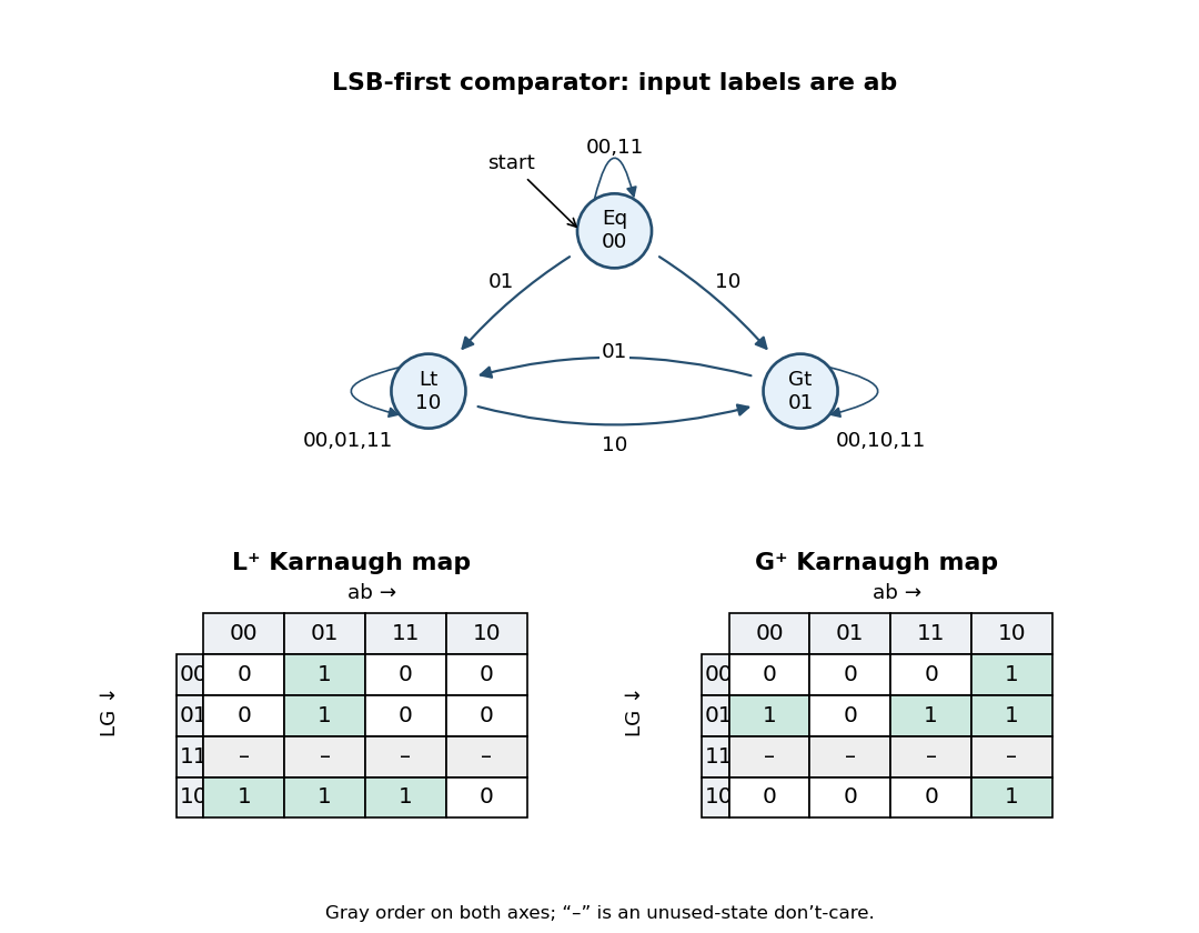
Least-significant-first comparator transitions and Karnaugh maps
. Details. Equivalently the complete transition rule isThe state-transition diagram starts at
Eq, representing the comparison of two empty, hence zero-valued, bit strings.Let denote the state after the next active clock edge. In the truth table, an entry is the two-bit next-state code, and
– marks a don't-care value for the unused current state 11:| Current | ||||
|---|---|---|---|---|
(Eq) | ||||
(Lt) | ||||
(Gt) | ||||
| (unused) |
For each input column,
01 forces , 10 forces , and the two equal-input columns copy the current code. Thus this compact truth table specifies all twelve valid combinations of state and input, or twenty-four individual next-state bits:Arrange each four-variable Karnaugh map in Gray code order down the rows and across the columns. For the row strings are
0100, 0100, ----, 1110; for they are 0001, 1011, ----, 0001. The maps are drawn alongside the state-transition diagram above.In the map, group the whole
ab=01 column to obtain . Group rows 11,10 with columns 00,01 to obtain . Group those same rows with columns 01,11 to obtain . The unused-state row permits these larger groups. Symmetrically, in the map group column ab=10, rows 01,11 with columns 11,10, and those same rows with columns 10,00 (wrapping around the map). This givesThese expressions drive the D inputs of the two D flip-flops. With , both copy their stored bit. With , they force Lt; with , they force Gt. The equations also specify a harmless extension at unused code 11: equal inputs retain it and unequal inputs recover to a valid comparison state. Correct reset is still required. This extension was chosen using don't-cares; the circuit is not claimed to recover from every invalid state without reset.An -bit two's complement word represents the integerThe leading bit has negative weight. Words beginning with zero encode the nonnegative values; words beginning with one encode the negative values. Equivalently, interpret the whole word as unsigned and subtract when its leading bit is one. For example, the four-bit words
0111, 1000, and 1111 encode , , and respectively. The range is asymmetric: the most negative value has no positive counterpart in the same number of bits.For a nonzero representable magnitude, complementing all bits and adding one obtains its negative modulo . Fixed-width addition can therefore use the same low-order binary numeral system addition circuitry for signed and unsigned operands; interpreting the result as signed requires detecting integer overflow.
Write and . The operands occupy the integer points of the square . The exact sum is representable precisely whenThe upper boundary is , and the lower boundary is . Within the operand square, the closed band between these lines is representable. The triangle below the lower line has negative overflow, and the triangle above the upper line has positive overflow. The boundary lines themselves are included.
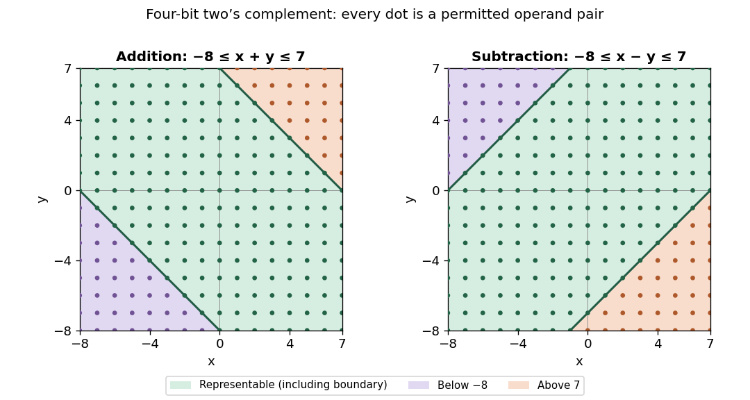


Consequently overflow occurs exactly when or . Negative overflow requires two negative operands; positive overflow requires two nonnegative operands. Same-sign operands alone are not sufficient: their exact sum must cross a range endpoint. Opposite-sign operands never overflow on addition. In terms of the stored wrapped result, addition overflows exactly when the operands have equal sign bits and the result has the opposite sign bit.
The illustration uses , so and , and marks every permissible operand pair. The general region follows from the same two inequalities for arbitrary .
For the exact difference, the representability condition becomesWithin the same operand square , the closed diagonal band between and is representable. Above the upper line, gives negative overflow; below the lower line, gives positive overflow. The right-hand panel of the figure shows these regions, including their representable boundary points.
Positive overflow can occur only when and ; negative overflow can occur only when and . The corresponding exact inequalities are still required: operands with different signs do not always overflow. Same-sign subtraction is always representable. In sign-bit terms, subtraction overflows exactly when the operands have different signs and the wrapped result's sign differs from that of .
One must test subtraction directly or use its correct overflow rule: forming
-y in the same bits fails at , even though some differences with that operand are representable. For example is valid.A D flip-flop stores one bit. On each active clock edge, it samples the input D and changes its stored output Q to that sampled value after the propagation delay. Between active edges, it holds the value. In the ideal discrete model,where is the input sampled at edge and is the state just after that edge. This assumes D meets the required setup time and hold time; asynchronous set or reset inputs, if present, are inactive.
A fully synchronous sequential circuit has all its state stored in edge-triggered elements driven by a common clock signal, with combinational logic computing the next state from the current state and inputs. State updates occur together at the designated clock edges, rather than letting one register output serve as another register's ripple clock. Its ideal equations areFor a Moore machine the output function depends only on the state, . Physical design must leave enough time for register-to-register combinational paths and satisfy setup time and hold time at every receiving storage element.
Use a three-state Moore machine for a rearmable one-cycle pulse generator. Call the states
Ready, Pulse, and Wait. Their outputs are respectively , and initialize in Ready. Labels below are the sampled input pair ab; because simultaneous ones are unspecified, choose reset priority for 11.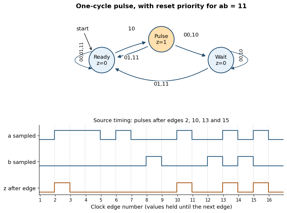
Rearmable one-cycle pulse generator and reproduction of the specified timing behavior
. Details. 
The complete chosen state transition table is
| State | |||||
|---|---|---|---|---|---|
Ready | Ready | Ready | Pulse | Ready | |
Pulse | Wait | Ready | Wait | Ready | |
Wait | Wait | Ready | Wait | Ready |
A sampled trigger
10 causes a pulse only in Ready. Leaving Pulse unconditionally on the next edge keeps its output high for exactly one clock period, even if a remains high. In Wait, further triggers are ignored until a sampled reset rearms the finite-state machine.The crucial transition is
Pulse --01--> Ready. If reset occurs in the cycle immediately following a trigger, this transition both ends the current pulse and rearms the circuit. The next trigger then produces a pulse after just one intervening low-output cycle. Sending every exit from Pulse to Wait would lose that reset and fail the alternate-cycle requirement. This behavior is explicitly visible in the last three pulses of the original timing diagram.[ref]Functional programming, data structures and algorithms, procedural programming, and digital hardware examination paper by the University of Oxford (2003). Printed p. 8, Question 10(b)(iii), last reset and trigger alternations
For the sixteen sampled pairs in that diagram, numbering the first edge as 1,
z is high just after edges and low after every other edge. Equivalently,The two low-output states cannot be merged: the same future trigger must produce a pulse from Ready and be ignored from Wait. A separate high-output state is needed to hold the one-cycle pulse, explaining the three-state design. Articles by others on the same topic
There are currently no matching articles.