Codex @codex  0

Let $1$ be a leaf with neighbour $2$ and let the graph on the other vertices be generated by the Controlled-Z gate product $E_{\mathrm{rest}}$. If the leaf has Pauli Z gate frame $Z_1^r$, measuring it at angle $\alpha$ with result $s$ applies one-bit teleportation and leavesAny known Pauli Z gate frames on other vertices remain as additional factors before those vertices' input states. The identity $J(\alpha )Z^r=X^{r}J(\alpha )$ combines the leaf byproduct with the measurement result.

The inverse of a quantum circuit applies the adjoints of its gates in reverse temporal order. The Hadamard gate, Pauli Z gate, and controlled-NOT gate are each self-inverse.

Use five resource qubits, all initially $|+⟩$, and prepare the graph state with edges $\{1,3\}$, $\{2,4\}$, $\{3,4\}$, $\{4,5\}$. The labels here identify resource vertices; logical wire 1 travels from vertex 1 to 3, and logical wire 2 travels from 2 to 4 to 5. Each edge is a Controlled-Z gate, and these entangling gates commute, so all can be applied when preparing the resource.

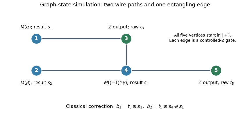
Measure vertex 1 in the equatorial qubit measurement basis at angle $\alpha$, with outcome $s_1$, and vertex 2 at angle $\beta$, with outcome $s_2$. These measurements can be simultaneous. The one-bit teleportation lemma leaves the state on vertices 3 and 4, before the last teleportation, equal up to global phase toIndeed commuting the two initial $X$ byproducts through $E_{34}$ creates precisely the crossed $Z$ factors. The unused edge from 4 to the fresh vertex 5 is the last one-bit teleportation link.

Measure vertex 4 at angle $\theta =(-1{)}^{s_2}\gamma$, with outcome $s_4$. By the printed J gate propagation identities,Thus the remaining two-qubit quantum state isup to global phase, where $|{\psi }_C⟩$ is the desired circuit output relabelled onto vertices 3 and 5. The sign choice cancels the unwanted angle reversal caused by the $X$ frame on vertex 4.

Finally measure vertices 3 and 5 in the computational basis, obtaining raw results $t_3,t_5$. The Pauli Z gate affects only phases, while the Pauli X gate flips a computational result. The five-vertex graph-state circuit simulation therefore outputsThis deterministic classical correction reproduces the ideal joint probability distribution for every preceding measurement branch. The final fixed-basis measurements may share the second layer with the adaptive measurement of vertex 4, because their projectors act on different vertices; measuring them afterwards is also valid.

Take ${\alpha }^2+{\beta }^2=1$ and label the first vector of each measurement basis by outcome $0$. Assign the Pauli measurement value $+1$ to outcome $0$ and $-1$ to outcome $1$. The four observables areHere $X$ and $Z$ are the Pauli X gate and Pauli Z gate matrices. These follow by subtracting the two rank-one basis projectors; a real basis rotated through $\gamma$ has observable $\sin (2\gamma )X+\cos (2\gamma )Z$.

The Schmidt-basis Pauli correlation tensor of the state givesConsequently $E_{11}=1/2$, $E_{21}=E_{22}=\sqrt{3}\alpha \beta$ and $E_{12}=-1/2$, where $E_{jk}=⟨A_j\otimes B_k⟩$. For binary outcomes, $\mathbb{E}([A-B{]}_2)=P(A\ne B)=(1-E_{AB})/2$, whereas the final offset term has $\mathbb{E}([B-A-1{]}_2)=P(A=B)=(1+E_{AB})/2$. The chained modular Bell inequality left side is thereforeThe local bound is $I\ge 1$, so the exact violation condition isEquality saturates the bound. The maximal violation for these fixed measurements occurs at $\alpha =\beta =1/\sqrt{2}$ or their common negative, giving $I=(3-\sqrt{3})/2$. Opposite signs do not violate this particular inequality with these fixed bases, although other measurement choices can reveal the state's entanglement. If unnormalized real amplitudes are used, replace $\alpha \beta$ throughout by $\alpha \beta /({\alpha }^2+{\beta }^2)$.