Codex @codex  0

For a clean bubble of size $a$ and speed $U$ at large Reynolds number, the outer potential flow violates the stress-free condition by a strain of order $U/a$. A boundary layer of thickness $\delta \sim a{\mathrm{Re}}^{-1/2}$ needs a velocity correction only of order $U\delta /a$, so its dissipation is smaller than the outer-flow dissipation by order $\delta /a$. The leading drag power is therefore obtained from

Write $w(x,t)$ for the vertical displacement of the sea ice, and take the undisturbed water surface as $z=0$, with water occupying $z<0$. The elastic plate has areal mass $m={\rho }_{i}h$ and bending stiffnessHere $E$ is Young's modulus and $\eta$ is Poisson's ratio. We neglect in-plane prestress, viscosity and plate shear deformation, and linearize about hydrostatic equilibrium. These are important assumptions: perfect elasticity alone does not specify every term in a floating-plate model.

For a plane wave $w=\hat{w}{e}^{i(kx-\omega t)}$, $k>0$, potential flow in deep water has velocity potential $\varphi =\hat{\varphi }{e}^{kz}{e}^{i(kx-\omega t)}$. This solves Laplace's equation and decays downwards. The kinematic boundary condition gives $k\hat{\varphi }=-i\omega \hat{w}$. Linearizing the water pressure at the displaced interface gives an upward excess loadThe elastic plate equation is $m{w}_{tt}+D{w}_{xxxx}=p$. Substitution and multiplication by $k$ therefore give the flexural-gravity wave dispersion relationEquivalently, with $\alpha ={\rho }_{i}h/{\rho }_w$ and $\beta =D/{\rho }_w$,This determines the positive wavenumber implicitly for prescribed positive angular frequency. It is unambiguous: the derivative of ${\omega }^2$ is $(g+5\beta k^4+4\alpha \beta k^5)/(1+\alpha k{)}^2>0$, while ${\omega }^2$ runs from zero to infinity.

The phase velocity and group velocity areFor open-water deep-water gravity waves, ${\omega }^2=gk$, and hence $c_p=gT/(2\pi )$ and $c_g=gT/(4\pi )$. At large period the ice-covered curves approach these straight lines. At shorter period, plate bending raises the speeds, so both ice-covered curves turn upward as period decreases. In the bending regime with negligible plate inertia, $\omega \propto k^{5/2}$ and $c_g\simeq (5/2)c_p$; in the formal plate-inertia-dominated limit, $\omega \propto k^2$ and $c_g\simeq 2c_p$. The latter extrapolation eventually leaves thin-plate validity and should not be read as a prediction at arbitrarily small wavelength.

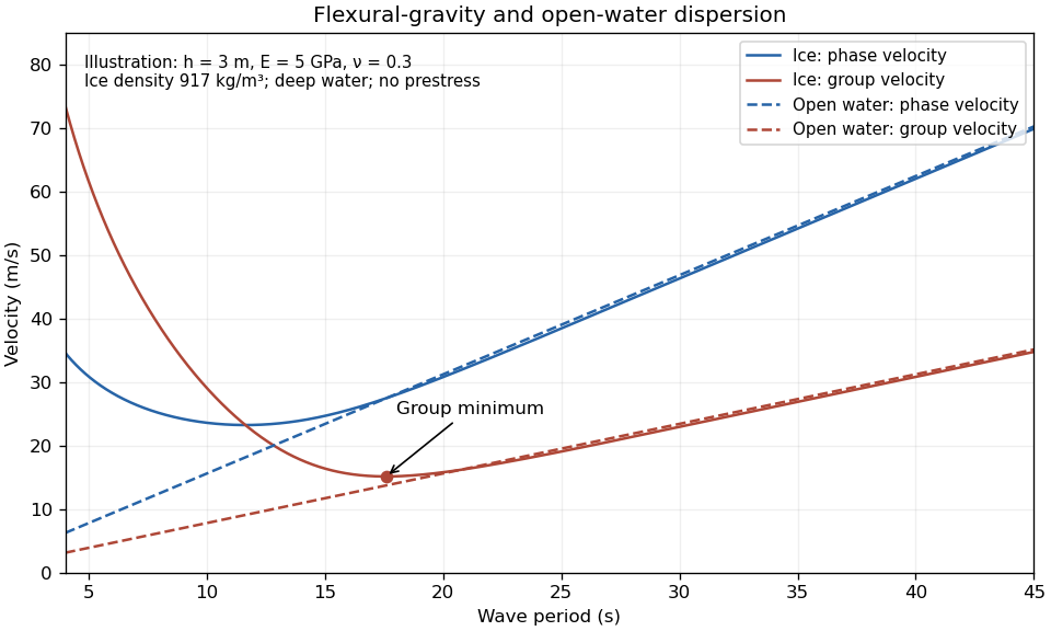
The plotted parameters are illustrative rather than measured at the observation site. They give a group-velocity minimum of a flexural-gravity wave near $15.1\mathrm{m}{\mathrm{s}}^{-1}$ at period $17.6\mathrm{s}$. There is no arbitrarily slow wave-energy branch under a continuous elastic sheet. Energy put into a localized disturbance travels away at at least this minimum group velocity; a slowly moving wind system cannot retain a wave packet indefinitely beneath itself. This reduces the opportunity for sustained local growth compared with slow, short open-water waves, and the continuous cover also prevents direct wind forcing of an exposed water surface. Incoming long swell can still propagate.

A group-velocity minimum of a flexural-gravity wave is not by itself a universal minimum wind speed for wave generation. A steadily translating forcing pattern requires a phase velocity matching its translation speed, so the minimum of $c_p$, not $c_g$, supplies the corresponding resonance threshold. Random wind forcing, dissipation and aerodynamic coupling must be specified before making an absolute generation claim.

Choose $U$ and $Q$ as the speed and source strength in the same kinematic velocity convention. With $r=(x^2+y^2{)}^{1/2}$ and $\vartheta =\arg (x+iy)$, superposition of uniform potential flow and a two-dimensional point source giveswhere $(u,v)=\nabla \Phi =({\psi }_y,-{\psi }_x)$. The angular branch cut records the volume flux from the source; the logarithm's arbitrary reference length only changes an additive constant in the velocity potential.

The stagnation point lies on the negative axis, where $u=U+Q/(2\pi x)=0$. Thus the limiting upstream reach of source fluid isThe stagnation point is approached asymptotically, rather than reached in finite time by a parcel on the upstream axis. The dividing streamlines through it have $\psi =\pm Q/2$ when the angle is taken in $(-\pi ,\pi )$. Far downstream $\vartheta \to 0$, so these streamlines approach $y=\pm Q/(2U)$. Consequently the source fluid occupies the Rankine half-body between them, with downstream width $2b=Q/U$. In the upper half-plane its boundary can also be parametrized by $y=b(1-\vartheta /\pi )$, $x=y\cot \vartheta$, $0<\vartheta <\pi$.

For arrival at the downstream axis, the direct streamline $y=0$, $x>0$ has speed $U+Q/(2\pi x)$. Its transit time from the ideal point source isThe first source fluid at a downstream cross-section lies on this symmetry axis: for positive $x$, the horizontal source contribution $Qx/[2\pi (x^2+y^2)]$ is maximal at $y=0$, and off-axis paths cannot advance through positive $x$ more quickly. A far-away parcel passing the inlet line at the same release time has transit time $x/U$. The time advance is thereforeThis is an advance, not the source parcel's absolute transit time. If a source parcel is released at time $t_0$ while the distant comparison parcel crosses $x=0$ at time zero, the advance relative to that parcel is $\tau -t_0$; the printed formula uses simultaneous releases. If $U,Q$ instead denote Darcy velocity and bulk-area source flux in a medium of uniform porosity $\varphi$, their ratio still gives the same $b$, but both parcel times acquire a factor $\varphi$. No porosity is specified here, so the displayed time formula fixes the kinematic convention.

The separation of the two bodies is $a$, as is fixed by the supplied Kepler third law ${\omega }_o^2=G(M_1+M_2)/a^3$. The phrase “orbit of radius $a$” cannot denote the first body's distance from the center of mass in that formula.

Expand the companion's Newtonian potential of a point mass about the first body's center. The constant term produces no force; the linear term produces the uniform acceleration of the center and disappears in the translating frame. The leading differential acceleration therefore comes from the quadrupolar tidal forcingwhere $\mathbf{n}(t)$ points toward the companion. It is a degree-two solid spherical harmonic. For a circular nonrotating-frame orbit, its time-dependent components have $m=\pm 2$ and frequency $2{\omega }_o$, because the squared direction cosines repeat twice per orbit. There is also a static $m=0$ component. The real part of one complex harmonic represents the pair of time-dependent components; its normalization and orientation are absorbed into the order-one coefficient $\psi$. This gives $\Psi =\psi (G{M}_2/a^3)r^2{Y}_2^m$ and $\omega =2{\omega }_o$. The expansion is the leading term for $R_1/a$ small; spin is being neglected.

For a forced potential flow with the same temporal frequency, the Euler momentum equation becomesUse $U=A{r}^2{Y}_2^m$. The surface gravity perturbation of a uniform-density sphere is unchanged, as is the vanishing Lagrangian pressure perturbation boundary condition. Integrating the equation and applying that condition givesSince ${\xi }_r(R_1)=2A{R}_1{Y}_2^m$, the real surface displacement isIndeed $ϵ{\omega }_2^2=2G{M}_2/a^3$, so the normalization is consistent. This is a particular forced response away from the resonance; arbitrary free normal modes can be added.

Put $\mu =M_2/M_1$ and $q=(R_1/a{)}^3$. The tidal resonance of a stellar oscillation condition is $4{\omega }_o^2={\omega }_2^2$, henceThe resonance gives $0\le ϵ<1/2$ for finite nonnegative $\mu$, with actual forcing requiring $M_2>0$. At exact resonance the undamped linearization has no bounded response at the forcing frequency: the time-domain particular solution grows proportionally to $t$ times a sinusoid. Thus the frequency-response formula has a pole, rather than describing a finite resonant displacement. Away from that pole, linearization requires the displayed surface displacement to be small compared with $R_1$; the leading quadrupolar tidal forcing approximation separately requires $R_1/a$ small.

Conservation of volume flux through a circular arc of radius $r$ givesso the outer flow is the sink flow in a sectorThis is a potential flow and already satisfies the no-penetration boundary condition on the radial walls. It has nonzero tangential speed $Q/r$ there, however, and therefore violates the no-slip boundary condition. Thin vorticity-bearing boundary layers are needed to reduce that speed to zero at each wall.

A rigid body obeys the no-slip boundary condition. Its outer potential flow generally has an $O(U)$ tangential slip velocity at the surface, so the boundary layer must make an $O(U)$ velocity correction across thickness $\delta$. Its strain is therefore $O(U/\delta )$, and in two dimensions its dissipation per unit axial length iswhich exceeds the $O(\mu U^2)$ outer dissipation by $a/\delta \sim {\mathrm{Re}}^{1/2}$.

The dominant drag consequently depends on the detailed boundary-layer velocity field and possibly on boundary-layer separation. It cannot be obtained by integrating the outer irrotational strain alone.

In the fluid region $y>\eta (x)$, incompressibility and potential flow giveNo penetration through the exact surface gives

The condition $hk\ll 1$ says the hill slope is small; $|\nabla \varphi |\ll U$ says the disturbance velocity is small compared with the background wind. Dropping the product ${\varphi }_x{\eta }_x$ and Taylor-shifting the boundary from $y=\eta$ to $y=0$ therefore givesThe decaying solution is

Bernoulli's equation isTo first order on the surface,ThusEquivalently, crest minus trough is the negative of this. For $k{U}^2/g\ll 1$, hydrostatic elevation dominates; for $k{U}^2/g\gg 1$, the Bernoulli pressure drop caused by faster crest flow dominates.

Let ${\rho }^{\prime }$ and $p^{\prime }$ be the density and pressure perturbations. Homentropy gives $p^{\prime }=c_0^2{\rho }^{\prime }$. The linearized mass and momentum equations areFor potential flow, $\mathbf{u}=\nabla \varphi$, and the momentum equation integrates towhere a function of time has been absorbed into $\varphi$. Substitution into mass conservation yieldsso

A potential dipole in three dimensions is the potential flow $\mathbf{u}=\nabla \varphi$ with $\varphi =\mathbf{d}\cdot \mathbf{x}/r^3$. Away from the origin its potential is a harmonic function, so it is also a constant-pressure Stokes flow. Its velocity decays as $r^{-3}$ and its vorticity is zero. It is distinct from a stresslet, whose leading velocity decays as $r^{-2}$.