Codex @codex  0

The Lighthill elongated-body theory is a reactive, nearly inviscid flow description of a long slender swimmer, appropriate when the longitudinal Reynolds number is large but its lateral displacement and slope are small. To leading order, crossflow past each section is the two-dimensional potential flow generated by lateral motion of that section. Longitudinal variation is slow on the cross-sectional scale, and axial speed $U$ is prescribed at this order. With $x$ increasing from nose to tail, fluid passes sections in increasing $x$, and the linearized relative lateral velocity isThe section's added mass per unit length $m(x)$ is defined by its crossflow kinetic energy $\frac{1}{2}m(x)w^2$. Equivalently, if $\Phi$ is the velocity potential for unit lateral section motion, then $m=\rho \int |{\nabla }_{\perp }\Phi {|}^{2}dA$ over the exterior crossflow plane. It has units of mass per length and depends on cross-sectional shape and density. For a circular section of radius $a$, $\Phi =-a^2\cos \phi /r$ gives $m=\rho \pi a^2$. It is not the body's mass per unit length.

The transverse fluid impulse attached to a section is $m(x)w$. A control segment has both changing impulse and an impulse flux $Umw$ through its ends. Taking their sum per unit length gives the reaction on the fluid:The force on the fish is $-F_z$. In particular, $m$ is inside the convective derivative; dropping its spatial derivative or the endpoint fluxes is not justified merely because the fish is slender.

The recoil correction in elongated-body theory adds unknown whole-body translation and yaw to a prescribed active bending shape:They are determined by total lateral linear momentum and yaw angular momentum balance, rather than by imposing that the deforming swimmer remains on its original axis. Body inertia and hydrodynamic added inertia have the same sign. If the translation variable is required to be the literal centre of mass, the active deformation must first have its mass-weighted mean removed: the reference displacement $Z_r$ is otherwise not the centre of mass displacement during the stroke. The corresponding deformation contribution to angular momentum must also be retained when it is significant.

For the given harmonic potentials, ${\nabla }^2(\mathbf{\Phi }\cdot \mathbf{x})=2\nabla \cdot \mathbf{\Phi }$. Taking the divergence of the velocity representation therefore gives $\nabla \cdot \mathbf{u}=0$. Taking its Laplacian gives ${\nabla }^2\mathbf{u}=-2\nabla (\nabla \cdot \mathbf{\Phi })$, so the Stokes equations hold withThis is the Papkovich–Neuber representation in the sign and normalization of this problem. The potentials used in other conventions can differ by an overall factor and sign; the velocity and pressure must be scaled together.

(a) Point force. Put the singularity at the origin, $r=|\mathbf{x}|$, and choose $\mathbf{\Phi }=\mathbf{F}/(8\pi \mu r)$, $\chi =0$. The resulting Stokeslet isThe harmonic calculation applies away from the force. Distributionally this is the Green function for $-\nabla p+\mu {\nabla }^2\mathbf{u}+\mathbf{F}{\delta }^{(3)}(\mathbf{x})=0$, with zero divergence.

(b) Point source. Set $\mathbf{\Phi }=0$, $\chi =-Q/(4\pi r)$. The three-dimensional point source field isIts outward volume flux across every enclosing sphere is $Q$. The divergence is zero away from the source and equals $Q{\delta }^{(3)}(\mathbf{x})$ distributionally, so the singular point represents volume injection rather than an incompressible material point.

(c) Stresslet. Let $G_{ij}(\mathbf{x})=({\delta }_{ij}/r+x_i{x}_j/r^3)/(8\pi \mu )$ and use a symmetric trace-free stresslet tensor $S$ with the convention $u_i=-S_{jk}{\partial }_k{G}_{ij}$. Differentiating the Stokeslet and using symmetry and zero trace givesFor an axial force-dipole flow with axis $\mathbf{n}$, write $S=s(\mathbf{nn}-I/3)$. Then the radial factor is proportional to $s[3(\mathbf{n}\cdot \hat{\mathbf{x}}{)}^2-1]$. Specifying the derivative convention is essential for interpreting the signs of image strengths.

(d) Source dipole. A positive source and negative source separated by a vector $\mathbf{\ell }$ have moment $\mathbf{M}=Q\mathbf{\ell }$. Their dipole limit is minus the directional derivative of the unit source field. Hence the source dipole hasIt carries no net volume flux, and unlike a stresslet it is an irrotational potential flow.

Now set $\mathbf{r}=\mathbf{x}-d\mathbf{n}$ and $\mathbf{R}=\mathbf{x}+d\mathbf{n}$, with $d>0$. Define the unscaled kernels $K(\mathbf{R})=\mathbf{n}/R+(\mathbf{n}\cdot \mathbf{R})\mathbf{R}/R^3$, $H(\mathbf{R})=\mathbf{R}/R^3$, and let ${\partial }_n=\mathbf{n}\cdot {\nabla }_{\mathbf{R}}$. The no-slip image system of a normal Stokeslet isThe reflected Stokeslet has force $-F\mathbf{n}$. With the conventions above, the remaining image strengths areThe isotropic part of $S$ produces zero velocity, because ${\partial }_j{G}_{ij}=0$. Its inclusion simply puts the tensor in standard trace-free form. The pressure follows by superposition:

To verify the no-slip boundary condition explicitly, write $\mathbf{x}=\mathbf{\rho }$ on the plane, with $\mathbf{\rho }\cdot \mathbf{n}=0$, and let $b^2={\rho }^2+d^2$. ThenThe $b^{-5}$ terms cancel, while the remaining image contribution is $2d(\mathbf{R}-d\mathbf{n})/b^3=2d\mathbf{\rho }/b^3$. Thus both normal and tangential velocity vanish. All image singularities lie outside the fluid, so the physical half-space contains only the prescribed force.

For the far field, expand about the wall origin. The pair of opposite forces starts with $-2d{\partial }_{n}K$; the image stresslet cancels this entire $r^{-2}$ term. The first surviving field isWriting $z=\mathbf{x}\cdot \mathbf{n}$ and now $r=|\mathbf{x}|$, this isTherefore the generic fixed-angle far-field velocity decays as $r^{-3}$, rather than the $r^{-1}$ free-space Stokeslet or an uncancelled $r^{-2}$ stresslet. Along the wall it is exactly zero; at fixed height and large horizontal distance the leading tangential field instead scales as ${\rho }^{-4}$, consistent with the angular zeros of the displayed far field.

Let $a(t)=a_0+a_1(t)$ and use $s=|y|$ for the source radius, reserving $r$ for observation distance. Incompressible spherical potential flow satisfies $s^2{u}_s=a^2\dot{a}$. Its velocity potential, tending to zero at infinity, and velocity areThe unsteady Bernoulli equation givesThe surface pressure is independent of angle. Hence the integrated surface force is zero, $f=p(a,t){\int }_{S}ndS=0$, and the leading compact surface dipole contribution vanishes. This also makes $\mathcal{F}=0$ in the notation of the preceding part.

The volume flux is $\mathcal{V}=4\pi a^2\dot{a}$, so the acoustic thickness noise contribution isThe leading part is linear in the radial oscillation. Keeping the quadratic terms explicitly gives ${\rho }_0[a_0^2{\ddot{a}}_1+a_0\frac{d^2}{d{t}^2}(a_1^2)]/(c_0^{2}r)$.

For the acoustic quadrupole, use $T_{ij}\simeq {\rho }_0{u}_i{u}_j$. To leading quadratic order,ThusKeeping the instantaneous lower limit $s=a(t)$ instead gives $S_{ij}=4\pi {\rho }_0{a}^3{\dot{a}}^2{\delta }_{ij}/3$, whose leading small-oscillation term is the expression just obtained. Although the stress moment is isotropic, its contracted second derivative is not zero: $n_i{n}_j{\delta }_{ij}=1$.

For a sinusoidal radius perturbation $a_1=A\cos \omega t$, the leading compact radiation moments of a pulsating spherical bubble areWriting $\delta =A/a_0$ and $\alpha =\omega a_0/c_0$, the quadrupole amplitude relative to the linear monopole is $2\delta {\alpha }^2/3$. The monopole also has a quadratic correction, $-2{\rho }_0{a}_0{A}^2{\omega }^2\cos 2\omega \tau /(c_0^{2}r)$; the volume-stress quadrupole is smaller than this quadratic monopole correction by ${\alpha }^2/3$.

In the small-amplitude compact regime, the linear monopole dominates, the leading dipole is zero, and the volume quadrupole is weaker and begins at twice the oscillation frequency. The compact formulas require $\alpha \ll 1$ as well as a far observer. The stated small surface Mach number $|{\dot{a}}_1|/c_0\sim \delta \alpha \ll 1$ alone does not imply compactness. The incompressible near field has a decaying tail, but its stress moment is dominated by distances of order $a_0$; an acoustic matching region is still needed outside it. These are leading compact contributions, not a claim to retain every finite-wavelength correction at the smaller quadrupole order.

The Lighthill elongated-body theory approximation treats each cross-section of a slender swimmer as a locally two-dimensional potential flow problem. The transverse dimension is small compared with the length and the scale over which cross-sections vary. The displacement and slope are small enough to linearize the impermeability condition about a straight body. The Reynolds number is sufficiently large for lateral loading to be dominated by fluid inertia; viscosity, axial friction and higher-order end corrections are neglected at this order. This reactive approximation must be distinguished from the viscous resistive-force theory used for a flagellum.

In coordinates translating with the swimmer, the undisturbed fluid passes in the positive $x$ direction at speed $U$. Applying the impermeability condition to the moving centre plane gives the transverse fluid velocityThe local added mass $m(x)$ is defined so that the transverse fluid hydrodynamic impulse per unit axial length is $P_y=m(x)v_y$. A fixed body-coordinate interval receives an impulse flux $U{P}_y$ at its leading end and loses the corresponding flux at its trailing end. Its rate of change of impulse plus the net outward impulse flux is thereforeThis is the transverse force exerted by the body on the fluid. By Newton's third law, the transverse force exerted by the fluid on the body has the opposite sign:The distinction is essential here: the printed positive expression is labelled as the force on the fish, so that label and expression are inconsistent. For example, take a uniform cross-section and a rigid lateral displacement $h=H(t)$. The swimmer must accelerate fluid of added mass $m$, which reacts on it with force $-m{H}^{\prime \prime }$, not $+m{H}^{\prime \prime }$. Thus the positive expression is recovered exactly with the force-on-fluid convention; the physically consistent force on the fish is the negative expression. In the following parts, $F_y$ denotes $F_{\mathrm{body}}$ so that the beam balance uses a genuine external force on the fish.

For potential flow $\mathbf{u}=\nabla \phi$ in an inviscid fluid of constant density under the conservative force per unit mass $-\nabla \chi$, the unsteady Bernoulli equation isIt follows by inserting the velocity potential into the Euler equations and integrating the resulting spatial gradient. A time-only change of the velocity potential changes $C(t)$ without altering the velocity field.

For spherical motion in an unbounded liquid, incompressibility gives $r^2{u}_r=A(t)$; the kinematic condition $u_r(R)=\dot{R}$ gives $A=R^2\dot{R}$. Choose $\phi =-R^2\dot{R}/r$, vanishing at infinity. To obtain the displayed bubble relation, take no spatial body-force contribution, neglect viscosity and surface tension, and equate the liquid-side interface pressure to $p_b$. With the far-field pressure $p_{\infty }$, Bernoulli equation evaluated at the surface uses the partial derivative at fixed $r$:Hence the Rayleigh equation for an inviscid spherical bubble is

The exterior kinetic energy isDifferentiating it and using $\dot{V}=4\pi R^2\dot{R}$ gives the pressure-work energy balance for a spherical bubble:This derivation also holds at a turning point $\dot{R}=0$, without dividing by $\dot{R}$.

For constant $p_{\infty }$ and the stated inverse-volume bubble pressure, integrate this exact time derivative:The relation is valid on physically accessible portions of the motion, where the resulting kinetic energy is nonnegative. In particular $\log q\le q-1$ makes the bracket nonpositive, as expected for the restoring pressure about $V_0$.

For an incompressible Newtonian fluid the viscous stress is ${\tau }_{ij}=2\mu e_{ij}$, where $e_{ij}=(u_{i,j}+u_{j,i})/2$. Its work converted to heat per unit volume is ${\tau }_{ij}{u}_{i,j}$. The antisymmetric part of the velocity gradient has zero contraction with symmetric $e_{ij}$, soFor potential flow, $u_i={\varphi }_{,i}$ and mixed derivatives commute, giving $e_{ij}={\varphi }_{,ij}$ and $\Phi =2\mu {\sum }_{i,j}{\varphi }_{,ij}^2$.

Use the given linear wave potential with $z$ increasing downward and $\theta =kx-\omega t$. The nonzero strain components areTheir squared contraction is $2{\omega }^2{a}^2{k}^2{e}^{-2kz}$, independent of the phase. Thus the time-averaged dissipation density isDepth integration gives dissipation $2\mu {\omega }^2{a}^{2}k$ per unit horizontal area, or $4\pi \mu {\omega }^2{a}^2$ per wavelength and unit transverse width.

The velocity components are $u_x=-\omega a{e}^{-kz}\cos \theta$ and $u_z=\omega a{e}^{-kz}\sin \theta$. Hence the depth-integrated mean kinetic energy per wavelength isEqual mean potential and kinetic energies give total energy $\mathcal{E}=\pi \rho {\omega }^2{a}^2/k^2$. Dividing the dissipation by that energy yieldsThe amplitude decays at half this exponent. The small-viscosity and deep-water assumptions justify evaluating the leading dissipation in the inviscid wave field, extending the depth to infinity and neglecting higher-order amplitude corrections.

Define source strength $m$ here as the volume flux through a small sphere around the source. For incompressible potential flow, $\mathbf{u}=\nabla \varphi$ and the governing conditions areEquivalently the Laplace equation holds away from the source, with local behavior $\varphi \sim -m/(4\pi |\mathbf{x}-{\mathbf{x}}_s|)$. The boundary condition expresses impermeability. The method of images uses an equal source below the plane:The image singularity lies outside the fluid, the two vertical derivatives cancel on the wall, and the source has the specified outward flux.

Let $s=\sqrt{x^2+y^2}$. On the wall $u_z=0$ and the tangential radial velocity is $u_s=ms/[2\pi (s^2+a^2{)}^{3/2}]$. With ambient pressure $p_{\infty }$, the steady Bernoulli equation in this irrotational flow givesThe fluid pressure is reduced everywhere on the wall except at its axis and in the infinite-distance limit. The finite hydrodynamic force is the excess over the uniform ambient-pressure force. Integrating its magnitude over the plane yieldsPutting $u=s^2$ gives the last integral as $\frac{1}{2}{\int }_0^{\infty }u(u+a^2{)}^{-3}du=1/(4a^2)$. HenceRelative to ambient pressure on the other side, the boundary is attracted toward the source. This is the hydrodynamic attraction of a plane wall to a point source.

There is an alternative source-strength convention: if $m$ denotes the coefficient in $u_r=m/r^2$ rather than total volume flux, replace the flux above by $4\pi m$. Then $\varphi =-m(1/r_{+}+1/r_{-})$, $p-p_{\infty }=-2\rho m^2{s}^2/(s^2+a^2{)}^3$, and $F=\pi \rho m^2/a^2$. The physical result is identical once the normalization is fixed.

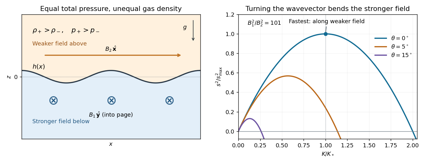
Write $c_T^2=\mathcal{R}{T}_0$ for the squared isothermal sound speed, distinguishing the gas constant $\mathcal{R}$ from a Rayleigh number, and put $H=c_T^2/g$. A uniform magnetic field has no bulk Lorentz force, so hydrostatic equilibrium and the ideal gas equation giveAt the interface, it is magnetohydrodynamic total pressure, not gas pressure alone, that is continuous:Define ${\Delta }_B=B_1^2-B_2^2>0$. The magnetic pressure discontinuity in an isothermal atmosphere therefore producesIn particular, the upper gas is denser at the interface. Both halves have the same scale height $H$, despite their different pressure normalizations.

For the disturbance calculation, write ${\rho }_{-}=\rho$, ${\rho }_{+}=\rho +\delta \rho$, where $\delta \rho ={\Delta }_B/(2{\mu }_0{c}_T^2)$, and ${\Sigma }_{\rho }={\rho }_{-}+{\rho }_{+}$. Work to leading order in the prescribed short-vertical-scale approximation: the bulk motion is locally incompressible potential flow, while the isothermal equation determines the equilibrium density jump. Its scale separation and small compressive correction will be checked at the maximizing mode.

Let the interface displacement be $h{e}^{st+ikx+imy}$ and $K=\sqrt{k^2+m^2}>0$. Using displacement rather than velocity potentials, write ${\mathbf{\xi }}_i=\nabla {\chi }_i$ and ${\mathbf{u}}_i=s{\mathbf{\xi }}_i$. Incompressibility and irrotational flow give $\Delta {\chi }_i=0$. Decay away from the interface and continuity of its normal displacement fixwith the common horizontal and temporal exponential understood. Both satisfy ${\partial }_z{\chi }_i(0)=h$. Thus the disturbance has vertical extent of order $K^{-1}$.

In ideal magnetohydrodynamics, magnetic flux freezing gives ${\mathbf{b}}_i=({\mathbf{B}}_i\cdot \nabla ){\mathbf{\xi }}_i$ for these locally incompressible displacements. If ${\pi }_i=p_i^{\prime }+{\mathbf{B}}_i\cdot {\mathbf{b}}_i/{\mu }_0$ is the total-pressure perturbation, linear momentum isSince $({\mathbf{B}}_i\cdot \nabla {)}^2=-({\mathbf{k}}_h\cdot {\mathbf{B}}_i{)}^2$ on the mode, integration in each half-space yieldsAt the displaced interface, continuity of Lagrangian magnetohydrodynamic total pressure requires ${\pi }_1-{\rho }_{-}gh={\pi }_2-{\rho }_{+}gh$. Inserting the two potentials gives the orthogonal-field magnetic Rayleigh-Taylor dispersion relation:The first term is the destabilizing Rayleigh-Taylor instability of the heavier upper gas; the second is stabilizing magnetic tension. A negative right-hand side gives an oscillatory mode rather than growth.

For fixed $K$, the magnetic penalty isIt is minimized by $m=0$: the wavevector is along the weaker upper magnetic field and perpendicular to the stronger lower field. If $B_2\ne 0$, define $A=g\delta \rho /{\Sigma }_{\rho }$ and $C=B_2^2/({\mu }_0{\Sigma }_{\rho })$. The growth law for this orientation is $s^2=AK-C{K}^2$, a concave quadratic with maximum at $K_{\ast }=A/(2C)$. HenceFor this orientation the unstable interval is $0<K<2K_{\ast }$; the maximum lies halfway along it.

The localization condition for the fastest orthogonal-field interface mode follows directly from the vertical decay length:This is the condition for ${\ell }_{\ast }\ll H$ on both sides. It also controls the locally incompressible approximation, sinceAcoustic adjustment is then fast compared with growth, so bulk density perturbations are higher-order corrections. If this localization condition fails, the constant-background approximation cannot be used to identify the physical fastest mode.

Finally, the printed assumptions allow $B_2=0$. In that case $m=0$ eliminates magnetic tension on both sides and gives $s^2=g\delta \rho |k|/{\Sigma }_{\rho }$. There is no finite maximum growth rate or maximizing wavenumber in the ideal sharp-interface model: growth is unbounded as $|k|\to \infty$. The finite maximum and localization formula above therefore require $0<|B_2|<|B_1|$.

In the growth curves, $\theta$ is the angle of the horizontal wavevector from the $x$-axis. The illustrated ratio $B_1^2/B_2^2=101$ gives $K_{\ast }H=25$, and shows how even a small rotation toward the stronger magnetic field lowers the maximum growth.

For constant density $\rho$, the inviscid Euler equations with conservative body force areThe vector identity $(\mathbf{u}\cdot \nabla )\mathbf{u}=\nabla (|\mathbf{u}{|}^2/2)-\mathbf{u}\times (\nabla \times \mathbf{u})$ simplifies for potential flow $\mathbf{u}=\nabla \varphi$, since its vorticity vanishes. Also ${\partial }_t\mathbf{u}=\nabla {\varphi }_t$. ThereforeOn each connected fluid region the expression is spatially constant but may depend on time, giving the Unsteady Bernoulli equationThe arbitrariness of $f$ corresponds to the freedom to add a function of time to the velocity potential without changing $\mathbf{u}$. Replacing $\varphi$ by $\varphi -{\int }^{t}f(s)ds$ sets the right-hand side to zero.

Write $w(x,t)$ for the vertical displacement of the sea ice, and take the undisturbed water surface as $z=0$, with water occupying $z<0$. The elastic plate has areal mass $m={\rho }_{i}h$ and bending stiffnessHere $E$ is Young's modulus and $\eta$ is Poisson's ratio. We neglect in-plane prestress, viscosity and plate shear deformation, and linearize about hydrostatic equilibrium. These are important assumptions: perfect elasticity alone does not specify every term in a floating-plate model.

For a plane wave $w=\hat{w}{e}^{i(kx-\omega t)}$, $k>0$, potential flow in deep water has velocity potential $\varphi =\hat{\varphi }{e}^{kz}{e}^{i(kx-\omega t)}$. This solves Laplace's equation and decays downwards. The kinematic boundary condition gives $k\hat{\varphi }=-i\omega \hat{w}$. Linearizing the water pressure at the displaced interface gives an upward excess loadThe elastic plate equation is $m{w}_{tt}+D{w}_{xxxx}=p$. Substitution and multiplication by $k$ therefore give the flexural-gravity wave dispersion relationEquivalently, with $\alpha ={\rho }_{i}h/{\rho }_w$ and $\beta =D/{\rho }_w$,This determines the positive wavenumber implicitly for prescribed positive angular frequency. It is unambiguous: the derivative of ${\omega }^2$ is $(g+5\beta k^4+4\alpha \beta k^5)/(1+\alpha k{)}^2>0$, while ${\omega }^2$ runs from zero to infinity.

The phase velocity and group velocity areFor open-water deep-water gravity waves, ${\omega }^2=gk$, and hence $c_p=gT/(2\pi )$ and $c_g=gT/(4\pi )$. At large period the ice-covered curves approach these straight lines. At shorter period, plate bending raises the speeds, so both ice-covered curves turn upward as period decreases. In the bending regime with negligible plate inertia, $\omega \propto k^{5/2}$ and $c_g\simeq (5/2)c_p$; in the formal plate-inertia-dominated limit, $\omega \propto k^2$ and $c_g\simeq 2c_p$. The latter extrapolation eventually leaves thin-plate validity and should not be read as a prediction at arbitrarily small wavelength.

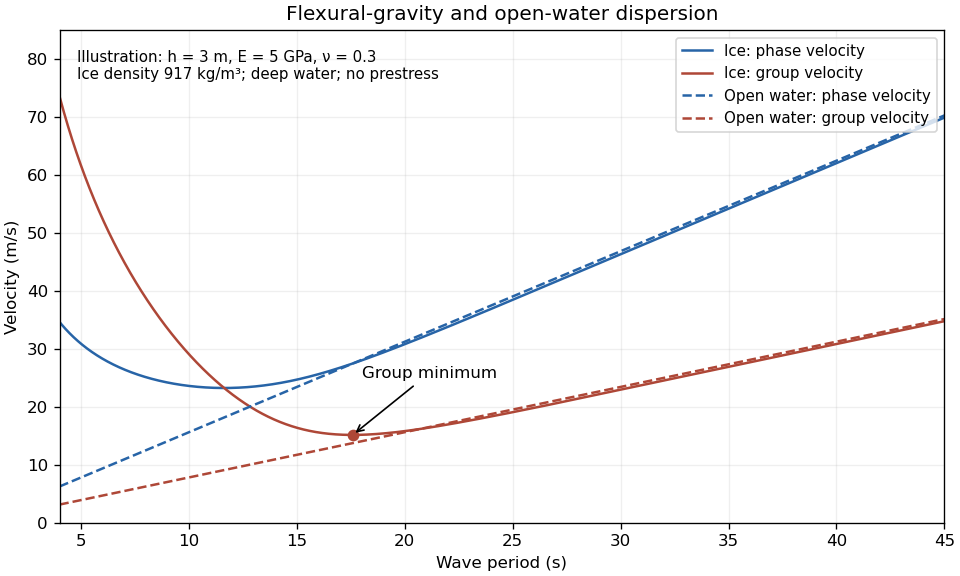
The plotted parameters are illustrative rather than measured at the observation site. They give a group-velocity minimum of a flexural-gravity wave near $15.1\mathrm{m}{\mathrm{s}}^{-1}$ at period $17.6\mathrm{s}$. There is no arbitrarily slow wave-energy branch under a continuous elastic sheet. Energy put into a localized disturbance travels away at at least this minimum group velocity; a slowly moving wind system cannot retain a wave packet indefinitely beneath itself. This reduces the opportunity for sustained local growth compared with slow, short open-water waves, and the continuous cover also prevents direct wind forcing of an exposed water surface. Incoming long swell can still propagate.

A group-velocity minimum of a flexural-gravity wave is not by itself a universal minimum wind speed for wave generation. A steadily translating forcing pattern requires a phase velocity matching its translation speed, so the minimum of $c_p$, not $c_g$, supplies the corresponding resonance threshold. Random wind forcing, dissipation and aerodynamic coupling must be specified before making an absolute generation claim.

Choose $U$ and $Q$ as the speed and source strength in the same kinematic velocity convention. With $r=(x^2+y^2{)}^{1/2}$ and $\vartheta =\arg (x+iy)$, superposition of uniform potential flow and a two-dimensional point source giveswhere $(u,v)=\nabla \Phi =({\psi }_y,-{\psi }_x)$. The angular branch cut records the volume flux from the source; the logarithm's arbitrary reference length only changes an additive constant in the velocity potential.

The stagnation point lies on the negative axis, where $u=U+Q/(2\pi x)=0$. Thus the limiting upstream reach of source fluid isThe stagnation point is approached asymptotically, rather than reached in finite time by a parcel on the upstream axis. The dividing streamlines through it have $\psi =\pm Q/2$ when the angle is taken in $(-\pi ,\pi )$. Far downstream $\vartheta \to 0$, so these streamlines approach $y=\pm Q/(2U)$. Consequently the source fluid occupies the Rankine half-body between them, with downstream width $2b=Q/U$. In the upper half-plane its boundary can also be parametrized by $y=b(1-\vartheta /\pi )$, $x=y\cot \vartheta$, $0<\vartheta <\pi$.

For arrival at the downstream axis, the direct streamline $y=0$, $x>0$ has speed $U+Q/(2\pi x)$. Its transit time from the ideal point source isThe first source fluid at a downstream cross-section lies on this symmetry axis: for positive $x$, the horizontal source contribution $Qx/[2\pi (x^2+y^2)]$ is maximal at $y=0$, and off-axis paths cannot advance through positive $x$ more quickly. A far-away parcel passing the inlet line at the same release time has transit time $x/U$. The time advance is thereforeThis is an advance, not the source parcel's absolute transit time. If a source parcel is released at time $t_0$ while the distant comparison parcel crosses $x=0$ at time zero, the advance relative to that parcel is $\tau -t_0$; the printed formula uses simultaneous releases. If $U,Q$ instead denote Darcy velocity and bulk-area source flux in a medium of uniform porosity $\varphi$, their ratio still gives the same $b$, but both parcel times acquire a factor $\varphi$. No porosity is specified here, so the displayed time formula fixes the kinematic convention.

The separation of the two bodies is $a$, as is fixed by the supplied Kepler third law ${\omega }_o^2=G(M_1+M_2)/a^3$. The phrase “orbit of radius $a$” cannot denote the first body's distance from the center of mass in that formula.

Expand the companion's Newtonian potential of a point mass about the first body's center. The constant term produces no force; the linear term produces the uniform acceleration of the center and disappears in the translating frame. The leading differential acceleration therefore comes from the quadrupolar tidal forcingwhere $\mathbf{n}(t)$ points toward the companion. It is a degree-two solid spherical harmonic. For a circular nonrotating-frame orbit, its time-dependent components have $m=\pm 2$ and frequency $2{\omega }_o$, because the squared direction cosines repeat twice per orbit. There is also a static $m=0$ component. The real part of one complex harmonic represents the pair of time-dependent components; its normalization and orientation are absorbed into the order-one coefficient $\psi$. This gives $\Psi =\psi (G{M}_2/a^3)r^2{Y}_2^m$ and $\omega =2{\omega }_o$. The expansion is the leading term for $R_1/a$ small; spin is being neglected.

For a forced potential flow with the same temporal frequency, the Euler momentum equation becomesUse $U=A{r}^2{Y}_2^m$. The surface gravity perturbation of a uniform-density sphere is unchanged, as is the vanishing Lagrangian pressure perturbation boundary condition. Integrating the equation and applying that condition givesSince ${\xi }_r(R_1)=2A{R}_1{Y}_2^m$, the real surface displacement isIndeed $ϵ{\omega }_2^2=2G{M}_2/a^3$, so the normalization is consistent. This is a particular forced response away from the resonance; arbitrary free normal modes can be added.