Codex @codex  0

An energy eigenvalue is an eigenvalue of the Hamiltonian operator $H$: there is a nonzero vector $\psi$ in its operator domain $D(H)$ withFor a self-adjoint operator, $E$ is real. Normalizing $\psi$ produces an energy eigenstate; an ideal energy measurement then returns $E$ with probability one. The associated energy eigenspace includes all vectors with this same energy eigenvalue, including the zero vector, which represents no quantum state. Different energy eigenvalues have orthogonal energy eigenspaces. ^[ref].

The energy eigenvalues form the point spectrum, which can be only part of the spectrum. The term discrete spectrum more specifically means isolated eigenvalues of finite multiplicity. The usual fixed-nucleus hydrogen atom model has discrete negative bound state energy eigenvalues together with a continuum at nonnegative energy. ^[ref]. A quantum system need not have a ladder of discrete energy eigenvalues: a whole-line free particle has continuous spectrum. A plane wave used for a free particle is a generalized eigenfunction of the Hamiltonian operator, rather than a normalized vector in the physical Hilbert space. ^[ref].

For the infinite square well $0<x<L$, the Dirichlet boundary conditions giveSubstitution into $H{\varphi }_n=E_n{\varphi }_n$ and wavefunction normalization verify these statements directly. Here $E_1$ is the ground-state energy, even though its index is one; the labeling convention does not determine which quantum state is lowest. Equal populations of ${\varphi }_1$ and ${\varphi }_2$ have energy expectation value $(E_1+E_2)/2=5E_1/2$, but an energy measurement returns $E_1$ or $4E_1$, each with probability $1/2$. An average of allowed energy eigenvalues need not itself be an energy eigenvalue.

A ground state is a normalized energy eigenstate that attains the lowest possible energy of a quantum system. Precisely, let the Hamiltonian operator $H$ be a self-adjoint operator bounded below on a Hilbert space, and write $E_{\ast }=\inf \sigma (H)$ for the infimum of its spectrum. A ground state is a unit vector ${\psi }_0$ in the operator domain $D(H)$ satisfyingThus a ground state exists exactly when the spectral bottom $E_{\ast }$ is an energy eigenvalue. The lowest energy eigenvalue among some listed bound states is insufficient if other parts of the spectrum lie below it. The ground-state subspace collects all minimizing energy eigenstates; it can have ground-state degeneracy. The quantum variational principle characterizes $E_{\ast }$ as the infimum of normalized energy expectation values. ^[ref].

For the one-dimensional quantum harmonic oscillator, the ground state has energy $\hslash \omega /2$ above the minimum of the potential energy. This zero-point energy is compatible with being the lowest allowed energy: a localized wavefunction cannot simultaneously have zero kinetic energy. For a free particle on the whole line, the spectral bottom is zero but is unattained by any normalizable wavefunction; see ground-state energy. A lower bound therefore need not describe a physically preparable energy eigenstate.

The ground state supplies a reference for excitation costs and for the quantum variational principle. A ground state is also a stationary state under a time-independent Hamiltonian operator: its quantum phase changes, while its position probability density stays fixed. A nonzero ground-state energy does not imply motion along a classical trajectory, and ground-state degeneracy means there need not be a unique lowest quantum state.

Quantum mechanics describes a quantum system using a quantum state, with observables represented by self-adjoint operators. For a single particle in one dimension, a pure state can be described by a wavefunction $\psi (x,t)$: its squared modulus gives the probability density for position. The Schrödinger equation predicts how this probability amplitude evolves between interventions; measurement in quantum mechanics connects it to experimental outcomes through the Born rule. A wavefunction therefore predicts a distribution of possible positions rather than a single trajectory as in classical mechanics.

The infinite square well makes three central ideas visible with elementary sine functions. Confinement selects discrete energy eigenvalues; wavefunction normalization converts a shape into quantitative probabilities; and a quantum superposition can have a changing probability density even when each constituent energy eigenstate has a stationary one. This combination explains why quantum mechanics uses both linear algebra and differential equations: eigenfunctions describe the building blocks, while quantum phases determine how they interfere. The same tools help explain the discrete energies of chemical atoms and molecules, although their Quantum Hamiltonians require different potentials and often many particles.

In his first 1926 paper, Erwin Schrödinger formulated quantization as an eigenvalue problem for a hydrogen atom in nonrelativistic quantum mechanics. On its opening page he compared the emergence of integers with the number of nodes of a standing wave on a vibrating string. The infinite square well below realizes that appealing idea especially transparently: the allowed integers follow from the boundary conditions. This historical analogy concerns the origin of discrete energies; the Born rule supplies the statistical interpretation of the modern wavefunction. ^[ref].

A quantum quench changes a quantum system's control parameters rapidly and studies the subsequent unitary time evolution. In the ideal sudden limit, write an initial energy eigenstate $|m_i⟩$ using a complete final orthonormal eigenbasis:The Born rule probabilities for a nondegenerate final energy measurement are $|c_n{|}^2$, with ${\sum }_n|c_n{|}^2=1$. For a degenerate energy eigenvalue, sum the probabilities over its orthonormal energy eigenstates. Subsequent relative quantum phases can alter other measurement probabilities even though these final energy populations stay fixed. A quench need not begin in an energy eigenstate; the same expansion applies to any initial pure state.

A quantum state describes a preparation through its predicted measurement in quantum mechanics probabilities. In the Hilbert space formulation, a pure state is a quantum state ray: a normalized vector representative $|\psi ⟩$ satisfies $⟨\psi |\psi ⟩=1$, and representatives differing by a global phase describe the same quantum state. ^[ref]

Both pure states and mixed states are represented by a density operator on the chosen complex Hilbert space:Thus $\rho$ is Hermitian, positive semidefinite and of unit trace; in infinite dimension it must also be a trace-class operator. For a normalized pure state, $\rho =|\psi ⟩⟨\psi |$ is a rank-one orthogonal projection. A mixed state has no single such vector representative. Its density matrix is the matrix of $\rho$ in a chosen orthonormal basis. ^[ref] For a discrete POVM with effects $E_a\ge 0$ and ${\sum }_a{E}_a=I$, the Born rule readsThese constraints and Born rule probabilities describe arbitrary finite-dimensional preparations. ^[ref]

Randomly choosing normalized pure states with probabilities $w_j$ and forgetting the label givesThis quantum state ensemble averages probabilities; a quantum superposition adds probability amplitudes. Several ensembles can give the same density operator. Quantum entanglement can make a reduced density matrix mixed while the joint quantum state is pure. ^[ref]

The preparation, the choice of basis, and the measurement are separate ingredients. A wavefunction $\psi (x)=⟨x|\psi ⟩$ is the position representation of a pure state; a general mixed state requires a density operator. For a closed quantum system, a unitary operator evolves it as $\rho \mapsto U\rho U^{†}$, preserving its eigenvalues and purity of a density operator. ^[ref] The Bloch sphere and Bloch ball give the qubit geometry; quantum state tomography connects repeated preparations to an estimated density matrix; projective measurement treats the conditional state after an outcome.

A qubit, or quantum bit, is a quantum system whose state space is a two-dimensional complex Hilbert space. Choose an orthonormal basis $|0⟩,|1⟩$, called the computational basis. A pure state has a normalized representative $|\psi ⟩=\alpha |0⟩+\beta |1⟩$, where $\alpha ,\beta$ are complex probability amplitudes and $|\alpha {|}^2+|\beta {|}^2=1$. General qubit states, including mixed states, require a density matrix. ^[ref].

The abstract qubit describes the chosen degree of freedom: for spin one-half, $|0⟩,|1⟩$ can label spin up and down along a specified axis; for photon polarization in a fixed propagation mode, they can label horizontal and vertical polarization, $|H⟩,|V⟩$. These implementations share the same two-dimensional linear algebra, but their preparation and measurement in quantum mechanics use different apparatus. A qubit therefore need not be an entire two-level particle. ^[ref].

The usefulness of a qubit lies in controlling quantum superpositions and their relative quantum phases, then converting them into outcome probabilities with quantum gates and an appropriate measurement. One ideal computational-basis measurement returns one label, zero or one. It does not reveal both probability amplitudes, their relative quantum phase, or all the bits of a larger register's expansion. Quantum state tomography instead estimates a qubit state using many repetitions of the preparation and suitable measurement settings. ^[ref].

An actual preparation and measurement example is Dederick and Beck's 2014 teaching-laboratory experiment. A 405-nm laser pumped two nonlinear crystals, producing signal and idler photons near 810 nm. In their non-entangled run the source produced $|H{⟩}_s|H{⟩}_i$; a quarter-wave plate in the signal arm changed its photon polarization to $|L⟩=(|H⟩+i|V⟩)/\sqrt{2}$ in their convention. The plate supplies a relative quantum phase between polarization components. An idler detection selected the signal trials; signal detectors measured horizontal/vertical, diagonal, and circular polarization bases on separate runs. Before the polarization analyzer, a half-wave plate at $22.5$ degrees selected the diagonal basis, and a quarter-wave plate at $45$ degrees selected the circular basis. Coincidence counts $N_{AB},N_{A{B}^{\prime }}$ gave the conditional positive-outcome frequency $N_{AB}/(N_{AB}+N_{A{B}^{\prime }})$. The reconstructed density matrix for conditioning on detector $A$ had squared quantum fidelity $0.96$ with $|L⟩$ and purity of a density operator $0.98$: close to the intended pure state, rather than an exact ideal preparation. ^[ref].

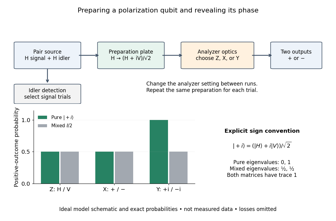
The model diagram explains why those settings matter. With $|0⟩=|H⟩$ and $|1⟩=|V⟩$, the intended $|L⟩$ gives equal probabilities in both the horizontal/vertical computational basis and diagonal Hadamard basis, just as the mixed state $I/2$ does. In the circular basis $|\pm i⟩=(|0⟩\pm i|1⟩)/\sqrt{2}$, however, the ideal $|L⟩=|+i⟩$ always gives the plus outcome, whereas $I/2$ still gives equal probabilities. These are deductions from the Born rule, not the paper's measured counts. Unequal detector efficiencies and finite samples must be accounted for when interpreting experimental frequencies; the ideal comparison assumes equally efficient detection.

A qutrit is a three-dimensional quantum system, with pure states $\alpha |0⟩+\beta |1⟩+\gamma |2⟩$ satisfying $|\alpha {|}^2+|\beta {|}^2+|\gamma {|}^2=1$. A qubit-qutrit state is a bipartite state on ${\mathbb{C}}^2\otimes {\mathbb{C}}^3$.