Codex @codex  0

Let $K_i$ generate Lorentz boosts with the same exponential convention as the rotation generators of rotations $J_i$. The Lie algebra of the Lorentz group isConsequently non-collinear Lorentz boosts do not close among themselves: the product contains a rotation, the Wigner rotation. For an explicit counterexample, in coordinates $(ct,x,y)$ write $c_a=\cosh a$, $s_a=\sinh a$ and similarly for $b$. ThenA pure rotationless Lorentz boost has a symmetric matrix, whereas this product has spatial entries $(xy)=0$ and $(yx)=s_a{s}_b\ne 0$ for $a,b\ne 0$. It is therefore a concrete product of two pure Lorentz boosts that is not a pure Lorentz boost. Collinear Lorentz boosts are the special case that do form a one-parameter group, with additive rapidities.

Allowing all spatial directions and closure generates both the $K_i$ and, through their commutators, all $J_i$. The smallest connected group containing all these Lorentz boosts is the proper orthochronous Lorentz groupIt contains arbitrary compositions of spatial rotations and Lorentz boosts continuously connected to the identity. It has six continuous parameters. Here “smallest” refers to the subgroup generated by all continuous pure Lorentz boosts, not to an arbitrary collection already including discrete reversals.

The full Lorentz group $O(1,3)$ has four connected components, distinguished by the sign of the determinant and the direction of time. Representatives are the identity, parity $P=\mathrm{diag}(1,-1,-1,-1)$, time reversal $\mathsf{T}=\mathrm{diag}(-1,1,1,1)$, and $P\mathsf{T}=-I$. ThusMultiplication by these discrete transformations relates the components algebraically; no continuous path within the Lorentz group joins different components. Translations are not required for closure here; adding them gives the larger Poincaré group.

The Euler-Lagrange field equation is $F^{\prime }(\varphi )-{\partial }_t^2\varphi +{\partial }_x^2\varphi =0$. ThereforePut $c=\cosh \beta$, $s=\sinh \beta$, $X=cx+st$ and $T=ct+sx$. The chain rule gives ${\partial }_t=s{\partial }_X+c{\partial }_T$ and ${\partial }_x=c{\partial }_X+s{\partial }_T$. Cross terms cancel and $c^2-s^2=1$, soThus the boosted scalar field is another solution for any constant rapidity. The nonlinear term in the nonlinear Klein-Gordon equation is unchanged because it is a local function of the scalar itself.

Use the amplitude placement in the original PDF: $w=[A{\cosh }^2(Bx){]}^{1/(1-n)}$. Introduce the actual peak $C=A^{-1/(n-1)}$ and $p=2/(n-1)$, so $w=C{\mathrm{sech}}^p(Bx)$. Its derivatives satisfyThe static equation is $w^{\prime \prime }=aw-b{w}^n$. Matching the constant and ${\mathrm{sech}}^2$ terms givesChanging the sign of $B$ leaves the profile unchanged. If $A$ is instead defined as an outside prefactor, as in the held TeX transcription, its value is $C$, not the PDF's $A$. This notation discrepancy does not change the physical profile.

The nonconstant positive power-law nonlinear Klein-Gordon pulse is even, smooth, has peak $C$ at zero and decays as $e^{-\sqrt{a}|x|}$. The requested sketches below compare several powers with illustrative $a=b=1$. For odd $n$, its negative is also a solution. A separate constant branch occurs for $B=0$: the positive equilibrium has $C=(a/b{)}^{1/(n-1)}$, or $A=b/a$ in the PDF convention. The zero solution is another equilibrium, obtained as a limiting profile rather than finite positive $A$.

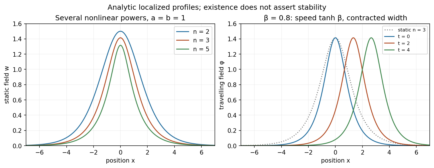
Now apply the Lorentz boost with rapidity $-\beta$ to the static field. It givesFor positive $\beta$, the centre moves to the right at $0<v<1$, with speed one the wave-speed unit. The peak stays $C$ and the width contracts by $1/\cosh \beta$. The shape translates without changing in time. This establishes a travelling solitary pulse; it does not by itself prove stability or elastic multi-pulse scattering.

A photon rocket converts stored mass-energy into a collimated beam of photons. In its instantaneous rest frame, energy conservation gives $c^{2}dM=-d{E}_{\gamma }$, and momentum conservation gives $Mcd\eta =d{E}_{\gamma }/c$. Therefore a monotone change in rapidity costs $M_f/M_i=e^{-|\Delta \eta |}$. The rocket's rest mass includes its fuel and stored internal energy; inefficiency or an angular spread of the exhaust increases the fuel requirement.

Accelerating from rest to rapidity $\eta$ and braking to rest requires two separate photon-rocket burns. Their mass ratios multiply, giving $M_f/M_i=e^{-2\eta }$. For ideal equal-mass matter–antimatter annihilation, the initial antimatter mass fraction is $(1-e^{-2\eta })/2$. Braking fuel must be carried and accelerated during the first burn.

For relativistic two-body scattering in one spatial dimension, this strip is the standard domain containing bound-state and crossed-channel poles. A stable-particle interpretation requires appropriate pole kinematics and residues; not every singularity automatically represents a new particle. Crossing relates rapidity $\vartheta$ to $i\pi -\vartheta$.

Rapidity is a dimensionless parameter for a signed collinear velocity $u$ with $|u|<c$, defined using the inverse hyperbolic functions byHere $c$ is the speed of light, and $\tanh$ is the hyperbolic tangent. Zero velocity has zero rapidity; negative velocity has negative rapidity. Every finite real rapidity gives $|u|<c$, while $u\to \pm c$ requires $\theta \to \pm \infty$. Thus a light ray has no finite rapidity in this parametrization. The header's formula uses natural units $c=1$: its $v$ is the numerical velocity $u/c$.

For the inertial frames in the velocity-addition formula, $S^{\prime }$ moves at signed velocity $V$ along the $x$-axis of $S$. Set $\varphi =\mathrm{artanh}(V/c)$. Re-expressing the same particle in the moving inertial frame givesThe subtraction is a passive change of reference frame; the inverse adds the particle's rapidity in $S^{\prime }$ to the frame's rapidity relative to $S$. For example, $V=0.6c$ and $u^{\prime }=0.6c$ give $\varphi ={\theta }^{\prime }=\ln 2$, so $\theta =\ln 4$ and $u=c\tanh (\ln 4)=15c/17$, exactly as in the velocity-addition formula.

For a massive particle of rest mass $m>0$ moving in one spatial dimension, its energy and signed momentum areThe hyperbolic cosine is the particle's Lorentz factor, and the hyperbolic sine is $\gamma u/c$. The hyperbolic Pythagorean identity immediately gives the relativistic energy-momentum relation $E^2-c^2{p}^2=m^2{c}^4$. In the older $c=1$ notation, writing the rest mass as $M$ recovers $v=\tanh \theta$, $E=M\cosh \theta$, and $p=M\sinh \theta$. These expressions use natural units in which the factors of $c$ are numerically one; the preceding formulas restore those factors explicitly. ^[ref].

The useful simplification follows from the hyperbolic-function identity $\tanh (a+b)=(\tanh a+\tanh b)/(1+\tanh a\tanh b)$: the nonlinear velocity-addition formula becomes ordinary addition of rapidities. See iterated collinear boosts with equal rapidity for a plotted example. A common collinear Lorentz boost shifts every rapidity by the same constant, so a rapidity difference is invariant. This makes rapidity useful for relativistic factorized scattering in one spatial dimension, where two-body S-matrices depend on the difference of the incoming rapidities, with particle species fixed.

For rectilinear motion write the four-velocity in an inertial frame as $U=(c\cosh \eta ,c\sinh \eta )$, where $\eta$ is the rapidity and $\tau$ is proper time. Differentiation gives $A=c\dot{\eta }(\sinh \eta ,\cosh \eta )$, with invariant $A\cdot A=-c^2{\dot{\eta }}^2$ in the $+-$ metric signature. The signed proper acceleration is therefore $a=c\dot{\eta }$. Constant signed acceleration gives $\eta ={\eta }_0+a\tau /c$; specifying initial position alone leaves the initial rapidity ${\eta }_0$ undetermined.

At relative rapidity $iu$, the analytically continued sum of the constituent four-momentum vectors is on the bound-state mass shell with the displayed mass. For equal constituents, rapidities $\chi \pm iu/2$ sum to $2m_a\cos (u/2)(\cosh \chi ,\sinh \chi )$. A pole at $u=0$ is at threshold rather than a strictly bound state.

The direct channel combines the two incoming four-momentum vectors. A one-particle pole in this channel has the intermediate particle's squared mass equal to $s$. Imaginary rapidity differences can satisfy this mass relation for a bound state even though there is no pole at real physical scattering rapidity.

For real parameters with ${\kappa }_i^2-b_i^2=1$, set $E_i=e^{{\kappa }_{i}x-b_{i}t+{\gamma }_i}$ and $a_{ij}=[({\kappa }_i-{\kappa }_j{)}^2-(b_i-b_j{)}^2]/[({\kappa }_i+{\kappa }_j{)}^2-(b_i+b_j{)}^2]$. Sum ${\prod }_i{E}_i^{{\mu }_i}{\prod }_{i<j}{a}_{ij}^{{\mu }_i{\mu }_j}$ over binary vectors of even parity for $f$ and odd parity for $g$. The Sine-Gordon equation solution is the continuous field $4\arg (f+ig)$. In the all-kink sector, ${\kappa }_i=\cosh {\theta }_i$, $b_i=\sinh {\theta }_i$ and $a_{ij}=-{\tanh }^2[({\theta }_i-{\theta }_j)/2]$. Treating these coefficients as positive would change the solution. Distinct rapidities give separated incoming and outgoing solitons.

For two equal-charge Sine-Gordon kinks with speeds $\pm v$, $0<v<1$, the positive spatial transition satisfies $X_{+}(T)=v|T|-\log v/(m\gamma )+o(1)$, where $\gamma =(1-v^2{)}^{-1/2}$. Labeling a soliton by its preserved rapidity, the right-moving incoming and outgoing intercepts differ by $-2\log v/(m\gamma )$. The soliton time delay at a fixed distant location is minus this shift divided by $v$, giving the displayed negative value. Reversing the entire field gives two antikinks with the same shifts. The sign means an advance relative to extrapolation of the incoming line; labels tied to left and right positions instead exchange velocities during reflection.

For the unit-modulus hyperbolic scattering block with elementary mass $m$, a pair bound at rapidity difference $iu$ has mass $m_2=2m\cos (u/2)$. Bootstrap fusion with another elementary particle gives a further direct pole at $3iu/2$. It is inside the physical rapidity strip with positive imaginary residue only for $0<u<2\pi /3$. In that range the new bound state has rest-frame constituent rapidities $iu,0,-iu$, so its energy is $m(1+2\cos u)=m\sin (3u/2)/\sin (u/2)$. Charges add at the bound-state vertex. At $u=2\pi /3$ the apparent pole cancels; beyond that point it lies outside the physical strip. The formula is conditional on this particular scattering block and its direct-pole interpretation, not a universal three-body binding law.

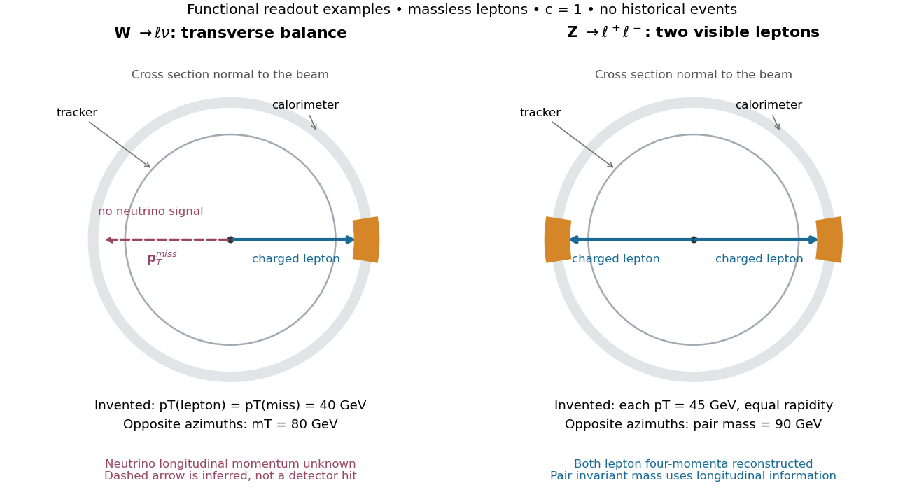
For a two-body W boson decay into a charged lepton $\ell$ and a neutrino, neglect both daughter masses and use natural units $c=1$. Let $\Delta \varphi$ be the angle between the daughter transverse momenta. Identifying the missing transverse momentum with the neutrino's givesThis observable uses no $p_{z\nu }$. The 1983 UA1 experiment paper already used transverse mass as a lower bound on parent mass, before making additional decay-model assumptions for a mass estimate.^[ref]

The bound follows directly from the energy–momentum relation. For each massless daughter write its four-momentum, using rapidity $y$ and azimuth $\varphi$, asUsing the Minkowski inner product with positive time sign, $p^2=E^2-|\mathbf{p}{|}^2$, the two daughter four-momenta give the true parent invariant mass $M$:Since $\cosh u\ge 1$, $m_T\le M$, with equality at equal daughter rapidities when both transverse momenta are nonzero. Thus the unmeasured longitudinal information can enlarge the true invariant mass, but cannot lower it below this ideal transverse mass.

For an original example, stipulate $p_{T\ell }=p_{T\nu }=40\mathrm{GeV}$ and $\Delta \varphi =\pi$. Then $m_T=80\mathrm{GeV}$. Equal rapidities give $M=80\mathrm{GeV}$; choosing $y_{\ell }-y_{\nu }=1$ with exactly the same transverse readout gives $M=80\cosh (1/2)\simeq 90.210\mathrm{GeV}$. One measured transverse configuration therefore permits different true parent masses.

For real $u$, this scalar S-matrix block satisfies $S_u(\theta )S_u(-\theta )=1$ and Hermitian analyticity of a two-particle S-matrix. It therefore has modulus one for real rapidity differences. For $0<u<\pi$ its pole at $\theta =iu$ has residue $2i\sin u$ and admits a direct-channel bound-state pole interpretation. Its crossed block is $\cosh [(\theta -iu)/2]/\cosh [(\theta +iu)/2]$. The endpoints $u=0$ and $u=\pi$ are removable degeneracies giving constant amplitudes, so a particle cannot be inferred there from the uncancelled denominator alone. This block specifies an amplitude; a complete theory must also obey the remaining crossing symmetry and bootstrap fusion constraints.

For the transmitting product with factors $\cosh [(\theta -i\pi j/N)/2]/\cosh [(\theta +i\pi j/N)/2]$ and prefactor $(-1{)}^N$, the continuous phase on $\theta \ge 0$ is $\pi N-2{\sum }_{j=1}^{N-1}\arctan [\tanh (\theta /2)\tan (\pi j/(2N))]$. Its derivative is $-{\sum }_j\sin (\pi j/N)/[\cosh \theta +\cos (\pi j/N)]$. A Riemann sum at fixed positive rapidity gives $(2N/\pi )\log \tanh (\theta /2)$ at leading order. The endpoints depend on the stated unwrapped branch; setting the high-energy value to zero silently changes the constant.

The velocity-addition formula translates a particle's velocity between two specified inertial frames. Let $S^{\prime }$ move at signed velocity $V$ along the $x$-axis of $S$, with parallel axes and $|V|<c$, where $c$ is the speed of light. Define $u_x=dx/dt$ and $u_x^{\prime }=d{x}^{\prime }/d{t}^{\prime }$ for the same particle's world line, using position and time measured within the corresponding inertial frame. With Lorentz factor ${\gamma }_V=(1-V^2/c^2{)}^{-1/2}$, the forward Lorentz boost gives

For collinear motion, write $u=u_x$ and $u^{\prime }=u_x^{\prime }$. The inverse velocity-addition formula isThis is the composition of the particle's velocity in $S^{\prime }$ and that frame's velocity relative to $S$. The velocities must belong to this same chain of reference frames, with directions specified. Two arbitrary quoted speeds cannot be inserted blindly. Each velocity measurement uses distances and clocks in a single inertial frame, with Einstein synchronisation for separated clocks.

For example, let $V=0.6c$ and let the particle travel at $u^{\prime }=0.6c$ in $S^{\prime }$. Its velocity in $S$ isThe Galilean transformation would instead give $u=u^{\prime }+V=1.2c$, which fails here. For light moving along the positive axis, $u^{\prime }=c$ gives $u=c$; $u^{\prime }=-c$ similarly gives $u=-c$. Negative directions also work for massive particles: at $V=0.6c$, $u^{\prime }=-0.6c$ gives $u=0$, while $u^{\prime }=-0.8c$ gives $u=-5c/13$. Thus “addition” means composition of signed velocities, rather than addition of their magnitudes.

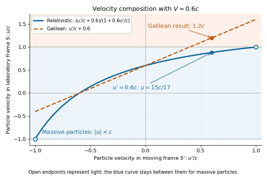
A short derivation differentiates the Lorentz transformation: $d{x}^{\prime }={\gamma }_V(dx-Vdt)$ and $d{t}^{\prime }={\gamma }_V(dt-Vdx/c^2)$. Dividing these differentials gives the longitudinal velocity-addition formula. The transverse formulas use $d{y}^{\prime }=dy$ and $d{z}^{\prime }=dz$, but the same transformed time denominator; omitting it would ignore the relativity of simultaneity. Replacing $V$ by $-V$ gives the inverse. When both relative and particle velocities are small compared with the speed of light, the denominator is close to one and the nonrelativistic limit recovers the Galilean transformation.

The formula lets us compare particle motion in a moving apparatus and a laboratory without losing the invariant speed of light. Einstein's 1905 paper derives the coordinate change in §3 and the composition of velocities in §5, including the collinear formula, its light-speed case, and composition of parallel transformations. ^[ref]. The rapidity parametrization makes the collinear composition particularly simple.

For two visible, approximately massless leptons, both measured four-momenta enterThis is a reconstructed invariant mass, including longitudinal information, rather than the lower bound obtained from transverse mass. As an original example, two opposite-azimuth leptons with $p_{T+}=p_{T-}=45\mathrm{GeV}$ and equal rapidities have $m_{\ell \ell }=90\mathrm{GeV}$. Changing their rapidity difference to one raises it to about $101.486\mathrm{GeV}$, even though their transverse momenta are unchanged.

The ideal transverse mass bound concerns the actual event's parent invariant mass, not a perfectly sharp universal number. A finite decay width spreads parent invariant masses; particle jet recoil changes daughter directions; invariant-mass resolution, momentum resolution and imperfect reconstruction can smear an observed endpoint. Recoil alone does not invalidate the ideal inequality when both daughter transverse momenta are correct. Additional invisible particles, radiated photons and a massless-daughter approximation can invalidate the simple two-body reconstruction. Likewise, a Z boson pair-mass peak requires control of identification, detection efficiency, instrumental response and backgrounds. A peak position and an endpoint are different summaries of selected event populations.