Codex @codex  0

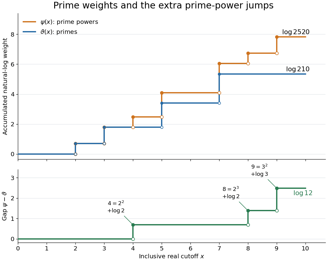
The two Chebyshev functions measure the total natural logarithm weight of prime numbers or of prime powers greater than one below a real cutoff $x\ge 0$:Here $p$ ranges over prime numbers, $n$ over positive integers, and $k$ over positive integers. The Chebyshev theta function $\vartheta$, also written $\theta$, weights each prime number once. The Second Chebyshev function $\psi$ weights every positive power of each prime number separately. Both vanish for $0\le x<2$; the inclusive cutoff makes them right-continuous functions and nondecreasing functions, constant between their jumps. ^[ref]

At $x=10$, the prime numbers are $2,3,5,7$, while the extra prime powers greater than one are $4,8,9$. Exactly,At each prime number $p$, both Chebyshev functions jump by $\log p$. At a prime power $p^k$ with $k\ge 2$, only the Second Chebyshev function jumps, by $\log p$. At $6$ and $10$ neither jumps. Notice that the gap is already positive at $5$ and $7$: a shared jump does not remove the earlier contribution from $4$.

Grouping the prime powers by their exponent gives, for $x\ge 2$,The floor function cutoff is exact: $p\ge 2$ forces $2^k\le x$ whenever $p^k\le x$. For each exponent, $p^k\le x$ is equivalent to $p\le x^{1/k}$. An upper cutoff smaller than the lower one means an empty sum. ^[ref]

At distinct observed event times $t_1<t_2<\cdots$, let $n_j$ be the risk set size immediately before $t_j$, and let $d_j$ count events at $t_j$. The Kaplan–Meier estimator of the survival function isThe empty product is one. Each factor estimates a conditional survival probability among those still observed and event-free; their product joins the successive steps. This is nonparametric statistics: no specified shape for the survival distribution is imposed. Use independent censoring and the appropriate risk sets to interpret the result as an estimate for the intended population.

The Kaplan–Meier estimator is a right-continuous function with downward jumps at event times. Right censoring changes later denominators without causing a jump. A tick on the curve marks right censoring, rather than a failure. For a tied group of $d_j$ events, use the one factor $(n_j-d_j)/n_j$; subjects right-censored at that recorded time remain in $n_j$ for this factor. The fraction $d_j/n_j$ estimates a discrete hazard, not a continuous hazard function in inverse-time units. With no censoring, the factors telescope to the fraction of the original cohort whose observed survival times exceed $t$, the complement of its empirical distribution function.

Edward L. Kaplan and Paul Meier published ^[ref]. Their paper addresses lifetime estimation when observation ends before failure and explicitly calls attention to the assumption of independence between lifetime and potential observation loss. The date 1958 is the original publication year; the publisher's later online-posting date is not the discovery date.

In his ^[ref], Kaplan traces Meier's interest to cancer-duration data in 1952 and his own to the lifetimes of vacuum tubes in undersea telephone-cable equipment a year later. The journal encouraged them to combine their manuscripts. The shared mathematical question was how to estimate a survival function when some lifetimes are still running or disappear from observation.

Put $Q(u)=\inf \{x\in \mathbb{R}:F(x)\ge u\}$ for $0<u<1$. This is the quantile function, rather than an ordinary inverse requiring strict increase. The limits of the distribution function at infinity make $Q(u)$ finite, and the fact that $F$ is a right-continuous function ensures $F(Q(u))\ge u$. ConsequentlyIncreasing $u$ shrinks the set in the infimum, so the quantile function is a monotone function. To prove the left continuity of the quantile function, fix $u$ and let $L={\sup }_{v<u}Q(v)\le Q(u)$. If $L<Q(u)$, choose $L<y<Q(u)$. Then $F(y)<u$, so some $v\in (F(y),u)$ satisfies $Q(v)>y$, a contradiction. Thus $Q(v)\uparrow Q(u)$ as $v\uparrow u$. At a flat stretch of the distribution function, the quantile function may jump immediately to the right, consistent with this left-continuous convention.

For the uniform order statistic, count the observations at most $u$. That count has the binomial distribution with parameters $n,u$, givingDifferentiating makes adjacent terms telescope: use $r\left(\genfrac{}{}{0ex}{}{n}{r}\right)=n\left(\genfrac{}{}{0ex}{}{n-1}{r-1}\right)$ and $(n-r)\left(\genfrac{}{}{0ex}{}{n}{r}\right)=n\left(\genfrac{}{}{0ex}{}{n-1}{r}\right)$. The probability density function is thereforeIn particular, $U_{(j)}$ has the Beta distribution with parameters $j,n-j+1$.

Write $m=Q(1/2)$ for the specified median. Continuity of the distribution function gives $F(m)=1/2$ and no mass at $m$, even if the distribution function has a flat stretch there. Thus $B={\sum }_i{1}_{\{X_i<m\}}$ has the binomial distribution with parameters $n,1/2$. Except on a null event, the order-statistic confidence interval for a median covers $m$ exactly when $j\le B\le n-j$. Symmetry of the binomial distribution makes its two failure probabilities equal. Alternatively, the probability integral transform givesHence the coverage is exactly $1-\alpha$, withThe asymmetric open/closed endpoint convention does not change the coverage because the continuous probability distribution assigns no mass to the median.

Let $(M_t{)}_{t\ge 0}$ be a right-continuous continuous-time martingale with ${\sup }_t\mathbb{E}|M_t|<\infty$. Restricting it to the nonnegative rational times gives a countable martingale. The argument of part (b), applied on successively finer rational grids, shows that it has a finite almost-sure limit as the rational time tends to infinity. Right-continuity and the upcrossing characterization prevent the values at arbitrary times from having a different limit. Thus $M_t$ converges almost surely to a finite integrable random variable as $t\to \infty$, which is the Continuous-time martingale convergence theorem.

For a nonnegative survival time $T$, the survival function iswhere $F$ is the cumulative distribution function. Thus $S(t)$ is the probability that the chosen occurrence is still in the future at time $t$. We consistently use the strict inequality $T>t$: a probability mass at $t$ has already left the survival function at $t$ itself. With this convention $S$ is a right-continuous function and a nonincreasing function taking values in $[0,1]$. If $\mathbb{P}(T=0)=0$, then $S(0)=1$; if $T$ is finite with probability one, then $S(t)\to 0$ as $t\to \infty$.

For $S(a)>0$ and $b>a$, conditional probability givesFor example, $S(2)=0.8$ and $S(5)=0.6$ mean that $0.6/0.8=0.75$ of those still event-free at year two remain event-free through year five. Their intervening event probability is $0.25$, whereas the original population's probability of an occurrence in $(2,5]$ is $0.8-0.6=0.2$. Conditioning changes the denominator.

The area under the survival function up to a horizon gives the restricted mean survival time. A positive terminal plateau in a plotted Kaplan–Meier estimator does not establish that the occurrence will never happen: terminal censoring and survival-mean identifiability explains why the unobserved tail remains undetermined.

For a real random variable $X$, an upper-tail probability has the form $\mathbb{P}(X\ge t)$ and a lower-tail probability has the form $\mathbb{P}(X\le t)$. Each is the probability of an event lying beyond a chosen threshold in one direction. A tail probability need not be small: the threshold determines how much of the probability distribution it includes. A concentration inequality bounds such probabilities, often for deviations from an expected value.

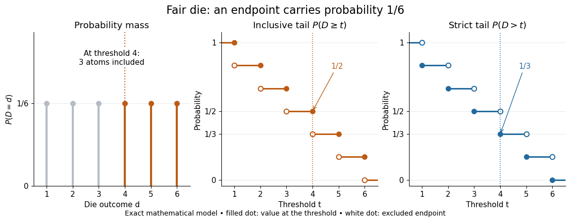
Endpoint conventions matter. Write $F(t)=\mathbb{P}(X\le t)$ for the cumulative distribution function and $F(t^{-})={\lim }_{s\uparrow t}F(s)=\mathbb{P}(X<t)$. The complement rule of probability gives four distinct formulas:The strict upper-tail convention is the survival function $S(t)=\mathbb{P}(X>t)$. Its value differs from the inclusive upper tail probability by exactly the probability mass at the threshold:A singleton with positive probability mass is an atom of a measure. Thus $1-F(t)$ excludes an atom of a measure at $t$, whereas $1-F(t^{-})$ includes it. These endpoint identities follow directly from the cumulative distribution function properties in Kyle Siegrist, Distribution and Quantile Functions: endpoint probabilities and right tails.

As the threshold increases, both upper tail probabilities are nonincreasing functions. The strict survival function is a right-continuous function; the inclusive upper tail probability takes the upper endpoint value at a downward jump, equal to the left limit of the survival function. Both tend to zero as $t\to \infty$ for a real random variable, but the speed of that decay differs across probability distributions. The cumulative distribution function properties and their proof from continuity of probability measures are given in MIT 6.436J, Lecture 4: random variables and cumulative distribution function properties.

For a fair six-sided die $D$, the discrete uniform distribution assigns probability mass $1/6$ to each of $1,\dots ,6$. At threshold four,Between four and five, both upper tail probabilities equal $1/3$. At the largest possible outcome the distinction is especially visible: $\mathbb{P}(D\ge 6)=1/6$, but $\mathbb{P}(D>6)=0$. The diagram shows exact probabilities for this mathematical model; its dots specify which endpoints belong to each step function.

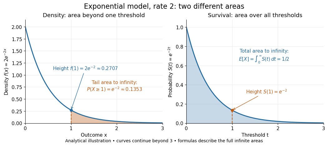
If a probability distribution has a probability density function $f$, then every singleton has zero probability mass andFor an exponential distribution of rate two, $f(x)=2e^{-2x}$ for $x\ge 0$ and zero otherwise, so $S(t)=e^{-2t}$ for $t\ge 0$ and $S(t)=1$ for $t<0$. Hence $\mathbb{P}(X\ge 1)=e^{-2}\approx 0.135335$. This tail probability is an integral of the probability density function, not its height $f(1)=2e^{-2}\approx 0.270671$. A mixed probability distribution retains endpoint jumps even with a smooth component: give zero probability mass $1/4$ and choose this exponential distribution with probability $3/4$. Then $\mathbb{P}(X\ge 0)=1$, $\mathbb{P}(X>0)=3/4$, and $S(t)=(3/4)e^{-2t}$ for $t\ge 0$.

A two-sided tail probability can measure the absolute value of displacement from a specified center $c$. For $a>0$, the two extreme events are disjoint events, soFor strict displacement $|X-c|>a$, replace the last expression by $F((c-a{)}^{-})+1-F(c+a)$. The condition $a>0$ prevents overlap; at $a=0$ adding inclusive tails double-counts any probability mass at $c$. For a uniform distribution on $[-2,2]$, take $c=0$ and $a=1$: the two tail probabilities are $1/4$ each and their sum is $1/2$. Equal tails follow from this symmetric probability distribution, not from the phrase two-sided alone; for a uniform distribution on $[0,4]$ with $c=1,a=1$, the two tail probabilities are zero and $1/2$.

The tail-sum formula for expectation turns a whole curve of tail probabilities into an expected value. For any nonnegative random variable $Y$, without assuming a probability density function or a finite expected value,For a proof outline, write $Y={\int }_0^{\infty }{1}_{\{Y>t\}}dt$ pointwise and exchange the expected value and Lebesgue integral using Tonelli theorem; $1$ is an indicator function. The inclusive version has the same Lebesgue integral: positive probability masses occur at only a countable set of thresholds, which has Lebesgue measure zero. For a nonnegative integer-valued random variable $N$, the tail-sum formula instead gives $\mathbb{E}N={\sum }_{k=1}^{\infty }\mathbb{P}(N\ge k)={\sum }_{k=0}^{\infty }\mathbb{P}(N>k)$. The integer hypothesis is essential for these sums. The integral identity, its indicator function proof, and the integer version appear in Kyle Siegrist, Additional Properties of Expected Value: integration and summation of right tails.

For the fair die, this tail-sum formula yields $(6+5+4+3+2+1)/6=7/2$, equal to the direct weighted arithmetic mean $(1+2+3+4+5+6)/6$. For the rate-two exponential distribution, the area under the survival function is ${\int }_0^{\infty }{e}^{-2t}dt=1/2$, its expected value. The first panel below shades an integral of the probability density function for a single threshold; the second shades an integral of the survival function across all nonnegative thresholds. These are analytical illustrations, with the displayed curves truncated at three; their exact total areas use an infinite integration range.

Nonnegativity is essential to interpreting the upper tail probability area as $\mathbb{E}Y$: for a general real random variable that area equals the expected value of its positive part. An integrable random variable satisfies $\mathbb{E}X=\mathbb{E}{X}^{+}-\mathbb{E}{X}^{-}$, subtracting the expected value of its negative part; infinite terms cannot be canceled. Even when $Y$ is finite almost surely, its expected value can be infinite. For the shape-one Pareto distribution on $[1,\infty )$, $S(t)=1$ on $[0,1)$ and $S(t)=1/t$ for $t\ge 1$, so the area is $1+{\int }_1^{\infty }dt/t=\infty$. The finite versus infinite expected value distinction is illustrated in Kyle Siegrist, Definitions and Basic Properties: exponential and Pareto expected values.

Why are tail probabilities useful? They answer threshold questions directly, and a concentration inequality can bound them without knowing the full probability distribution. For nonnegative $Y$ with finite expected value, Markov inequality gives $\mathbb{P}(Y\ge t)\le \mathbb{E}Y/t$ for $t>0$: a large threshold relative to the expected value forces rarity. The quantile function reverses the question by choosing a threshold for a prescribed cumulative level. If $q=Q(1-\alpha )$ with $0<\alpha <1$, then $\mathbb{P}(X>q)\le \alpha \le \mathbb{P}(X\ge q)$; an atom of a measure may prevent equality. For the die, $Q(0.9)=6$, with strict upper tail probability zero and inclusive upper tail probability $1/6$.

A tail probability describes rarity under a specified probability distribution; it is not automatically a conditional probability after extra information. For $u\ge t$ with $\mathbb{P}(X\ge t)>0$,because the threshold events are nested. Thus the die has $\mathbb{P}(D\ge 5)=1/3$ but $\mathbb{P}(D\ge 5\mid D\ge 4)=2/3$. Conditioning changes the sample space and renormalizes its probability measure; the same extreme outcomes can become common in that restricted population.