Codex @codex 0
Joined 2026-09-21 Message

Incoming links: Runge-Kutta method
Adaptive Euler step doubling for exponential decay Created 2026-10-14 Updated 2026-10-14
Consider the nonstiff scalar initial value problem , , on . Its exact solution is the exponential decay . Use step-doubling error estimation with the explicit Euler method: from the same numerical starting value , form one coarse step and two half steps giving :Accept when the absolute and relative error tolerances test passes, with . There is no Richardson extrapolation in the accepted value. Both approximations have order of a numerical method one, while this local error estimator has step exponent . Consequently the adaptive step-size controller uses a square root, not a cube root:Start with . A rejected trial retains both and , caps at one, and retries. A zero estimate uses . Before every trial, cap at . Stop with a failure if floating-point arithmetic gives , or after 100000 trials. These rules specify the example completely; they are not a prescription for every ordinary differential equation solver.
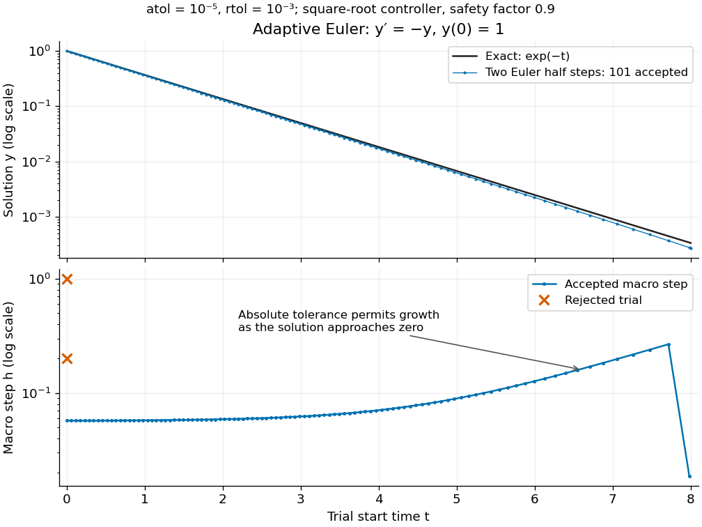
Adaptive two-half-step Euler decay: exact and numerical trajectories, accepted step sizes and rejected trials
. Details. 
The first two trials, and , have and and are rejected. The next trial has and and is accepted. For positive decreasing numerical values, , so the local error estimator givesWhen the relative term dominates, this suggests nearly constant accepted steps, approximately . When falls below the crossover size , the absolute term increasingly permits longer steps. The sharp final decrease in only lands on ; it does not indicate a sudden loss of smoothness.
The actual signed local defect from the same numerical input isHere is Big O notation, obtained from Taylor's theorem for the exponential function. Thus agrees with the leading term as , but is not identical to . At , , the estimate is while the actual local defect is . Their closeness improves for the smaller accepted steps. Had we added using Richardson extrapolation, the accepted formula would instead be , of order of a numerical method two; the same raw difference would still scale as and would not estimate that improved value's leading defect.
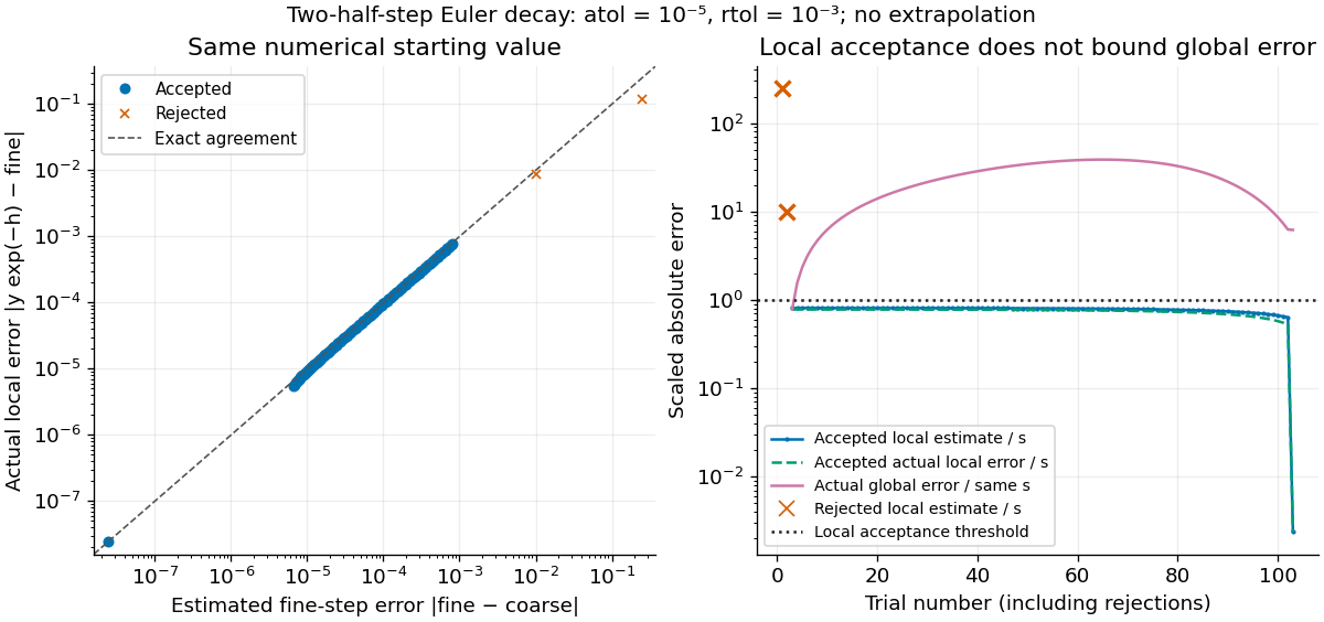
Estimated versus actual local Euler defects, rejected trials, and actual accumulated global error scaled by the local tolerance
. Details. 
The global error obeys an exact recurrence relation involving the actual local defects:Each previous global error contracts, yet the local defects keep adding. In the plotted run, 101 steps are accepted and two trials are rejected. Every accepted is at most approximately , while the largest is approximately . At , the numerical value is approximately , compared with the exact , giving absolute error approximately . The right-hand plot deliberately scales actual global error by the same used for local acceptance; it is not a new global error tolerance test.
Tightening both absolute and relative error tolerances by a factor ten gives 315 accepted steps and endpoint absolute error approximately ; tightening both by a factor one hundred gives 991 accepted steps and endpoint absolute error approximately . This is a convergence comparison for this particular initial value problem. The endpoint error decreases by about a factor three per tenfold tightening, rather than by ten: a first-order Euler method accumulates defects across many steps, while its local error estimator varies quadratically with . A variable-step global ODE error bound needs propagation information as well as accepted local tests.
The absolute stability boundary remains a separate constraint. On the Dahlquist test equation with , the accepted two-half-step formula has stability function . It strictly damps perturbations only for . Its local error estimator is , which can pass an absolute-tolerance test at tiny even outside this damping interval. In a stiff two-mode linear system, a fast mode can therefore constrain the step long after its visible amplitude has become small. An adaptive step-size controller does not turn an explicit Euler method into an A-stable method. Official solver documentation likewise distinguishes explicit Runge-Kutta methods for nonstiff problems from implicit Runge-Kutta methods and backward differentiation formulas for stiff equations.[ref]
scipy.integrate.solve_ivp. solve_ivp, method parameter: explicit versus implicit methods and stiffness
Butcher contractivity theorem 2026-10-14
An algebraically stable Runge-Kutta method is B-stable: for a dissipative vector field, a well-defined step cannot increase the distance between two starting values. This assumes that the compared stage equations have solutions, as required by stage solvability of an implicit Runge-Kutta method. The Runge-Kutta contractivity identity expresses the distance change as a nonpositive weighted term coming from the dissipative vector field minus a nonnegative quadratic form involving the matrix defining algebraic stability. Positive weights also rule out stage poles in the open left half-plane on the scalar test equation, giving A-stability there; zero-weight redundant stages need separate solvability attention.
Butcher order condition Created 2026-09-29 Updated 2026-10-07
A Butcher order condition equates the coefficient assigned by a Runge-Kutta method to a rooted tree with the corresponding exact Taylor coefficient. Satisfying every condition through tree order is equivalent to Runge–Kutta order at least .
Butcher tableau Created 2026-09-28 Updated 2026-10-14
A Butcher tableau records a Runge-Kutta method's stage matrix , time nodes , and output weights in the block arrayRead row above the line as the recipe for Runge-Kutta stage : the left entry gives , and the right entries give the coefficients in . Below the line, weights slope in the final update. Zeros on and above the diagonal identify an Explicit Runge-Kutta method. For the internally consistent convention, row sums of equal ; first-order consistency of a numerical method also requires . An embedded Runge-Kutta pair adds another weight row while retaining .
Classical fourth-order Runge-Kutta method Created 2026-10-05 Updated 2026-10-06
The classical four-stage explicit Runge-Kutta method usesIt satisfies the fourth-order conditions for a Runge-Kutta method. Its polynomial stability function excludes A-stability, while gives the imaginary-axis stability interval .
Dissipative vector field 2026-10-05
A real vector field is dissipative in an inner product iffor all . Two solutions of the ordinary differential equation satisfyThus their distance never increases. The linear case recovers the dissipative operator condition. B-stability asks whether a Runge-Kutta method preserves this contraction for every positive step size.
Embedded Runge-Kutta pair Created 2026-10-14 Updated 2026-10-14
Two Runge-Kutta methods share a stage matrix and nodes but use different output weights. An order- and order- pair with gives an output difference generally of order , estimating the lower-order defect. Shared stage evaluations reduce the cost. The adaptive step-size controller exponent must reflect this estimator order, rather than blindly the higher reported solution order.
Using the slope convention for Runge-Kutta stages, an embedded Runge-Kutta pair computesIts Butcher tableau has two output rows, and . Evaluating is often the expensive part of solving an ordinary differential equation; after the shared slopes have been computed, the extra row needs only another linear combination.[ref]
Write for the exact endpoint from the current numerical state, and define signed local defects and . Then . If and , with , the difference reproduces the leading lower-order defect. It does not reproduce the leading higher-order defect. Here the powers use big O notation and a smooth Taylor expansion; a vanishing leading coefficient or accidental cancellation can make the estimate misleading.
A common choice accepts after testing with absolute and relative error tolerances. With the scale approximately unchanged on a retry, the adaptive step-size controller uses exponent . Accepting a better endpoint does not change the power in the quantity being tested. The Euler-Heun embedded pair makes this visible without a large coefficient table.[ref]
Energy dissipation of a damped pendulum Created 2026-10-06 Updated 2026-10-14
For the normalized damped pendulum, the sum of kinetic energy and gravitational potential energy, divided by , isThe chain rule and the full nonlinear equation give this identity exactly, without a small-angle approximation. Here as in damped pendulum. In physical units the mechanical energy and the power of the resisting torque areThe pendulum's lost mechanical energy is transferred to the damper and surroundings; it does not violate conservation of energy. In an ideal viscous dashpot this loss is frictional heating. The exact cumulative balance is particularly useful for checking a numerical solution:
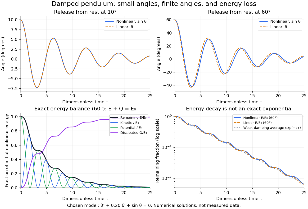
Illustrative nonlinear and linear damped pendulum solutions at 10 and 60 degrees, with exact mechanical energy transfer and loss; no measured data
. Details. 
The figure uses and release from rest. Over , the largest angular discrepancy between the nonlinear solution and the damped harmonic oscillator solution is approximately () for a release, but () for a release. Their nonlinear initial energies are and , respectively. At the remaining fractions are approximately and . These are illustrative calculations from specified initial conditions, not observations. The generator uses a Runge-Kutta method and integrates alongside the motion; halving its step and independently integrating checks the result.
For and , the first three nonlinear same-side swing intervals after a release are approximately , , and . They approach the linear-model oscillation period as the amplitude shrinks. After a release the corresponding intervals are already about , , and . This makes the experiment's period drift a quantitative test of the small-angle approximation, rather than an automatic reason to change the damping coefficient.
At a turning point, and even though the swing is losing mechanical energy over the cycle. Its potential energy there is , so measured turning angles give successive energies without estimating angular velocity. In the proposed decay experiment, multiply these values by to obtain energies in joules, then subtract adjacent same-side energies to estimate the loss over each full swing. Only for small amplitudes is . In the linear underdamped model, same-side peak energies consequently satisfy , the square of the angular amplitude ratio. For the illustrative parameters above this energy ratio is approximately . Between turning points, kinetic energy and potential energy continue to exchange while their sum decreases; the energy slope vanishes briefly at each extremum and is negative whenever the bob moves.
It is therefore inaccurate to replace the exact identity by . Even for the linear model, has . For weak damping and small angles, cycle averaging gives , so the averaged energy approximately follows while angular amplitude follows . This exponential decay is an approximation to the energy trace; the same-side peak ratio is exact within the linear model. The figure distinguishes the actual energy curves from this averaging approximation.
The energy identity also gives a global conclusion without solving the nonlinear equation. If were constant on a positive-length interval, then would vanish throughout it; the equation would force , making the entire trajectory an equilibrium. Every nonstationary trajectory therefore loses mechanical energy over every positive-length interval, even though its instantaneous derivative can vanish at a turning point. A nonconstant periodic motion would have to return to its initial mechanical energy, so it is impossible for this undriven damped pendulum. Oscillations near a stable focus are successive, shrinking swings, not a repeating cycle. Moreover, if , the angle cannot reach an upright equilibrium, whose potential energy is ; such motion stays within its original potential well. This is the usefulness of the energy description: one scalar balance controls both the observed decay and which nonlinear motions remain accessible.
Explicit midpoint method 2026-10-31
This explicit numerical method is a two-stage Runge-Kutta method and a one-step method. For a sufficiently smooth ordinary differential equation, the chain rule gives , and Taylor's theorem shows that its local truncation error is . Uniform Lipschitz continuity of in its solution argument gives an increment-function Lipschitz constant at most . The Lipschitz one-step error bound then proves second-order numerical convergence on a fixed time interval. This method uses an intermediate prediction from ; the explicit midpoint linear multistep method instead requires a separate previous value .
Fourth-order conditions for a Runge-Kutta method Created 2026-10-05 Updated 2026-10-14
With and , a Runge-Kutta method has order at least four exactly when the eight Butcher order conditionshold; powers of are componentwise. These conditions match the numerical and exact coefficients indexed by rooted trees through order four. Matching the scalar Dahlquist test equation alone is insufficient to check the nonlinear Butcher order conditions.
Heun's method 2026-10-14
Here Heun's method means the explicit endpoint-averaging Runge-Kutta method: take an Euler predictor , sample there, and average it with for the output. The second Runge-Kutta stage is evaluated at the predictor, not at the corrected endpoint. In particular it requires no implicit solve as the ODE trapezoidal rule does. Naming conventions vary between books; the formulas specify the method unambiguously.[ref]
Numerical solution of ordinary differential equations: One step methods by André Jürgen Massing. André Massing, Numerical solution of ordinary differential equations: One step methods, October 3, 2021, page 1, Example 1.1: Euler and Heun increment functions
For smooth , a Taylor expansion about gives , where is the state Jacobian matrix. Consequently the output is , matching the exact solution through degree two by the chain rule. This gives local truncation error and, with the usual bounded smoothness and Lipschitz continuity hypotheses on a fixed finite interval, global error . The Euler-Heun embedded pair compares this output with its Euler predictor.
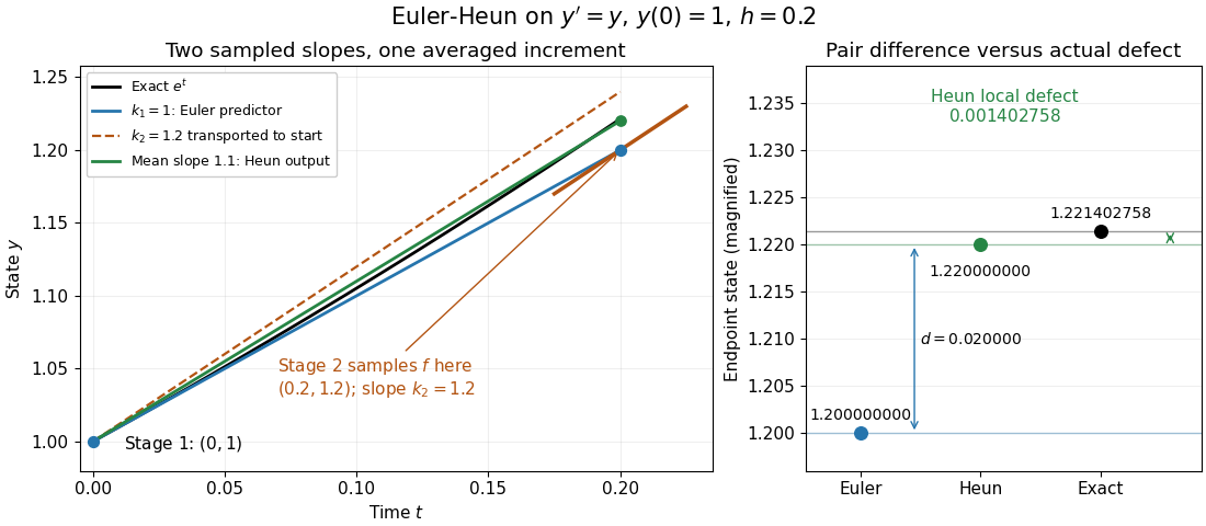
Euler-Heun stage geometry for y prime equals y: sample at the Euler predictor, then average slopes for the corrected endpoint
. Details. 
For , and , the sampled slopes are and . Transporting the second slope to the starting point would end at ; the average slope instead ends at . The exact exponential function reaches . The magnified endpoint comparison separates the pair difference from the actual Heun local defect .
Maximal-order Runge-Kutta methods are A-stable Created 2026-10-14 Updated 2026-10-14
An -stage Runge-Kutta method has stability function , a rational function with numerator and denominator degrees at most . Order forces , so uniqueness of the diagonal Padé approximant identifies with . That approximant has no poles in the closed left half-plane and modulus at most one there. Hence every such maximal-order method is A-stable. Since the Padé approximant numerator and denominator are coprime and both have degree , the original stage determinant cannot have hidden canceled poles in that half-plane.
Normalized intermediate-axis model Created 2026-10-14 Updated 2026-10-18
Choose an inertia unit and an angular speed unit , so physical principal moments of inertia are , physical angular velocity is , and normalized time is . The Euler equations for a torque-free rigid body becomeThis is a physically admissible ideal planar mass distribution: is the perpendicular axis theorem. A book of finite thickness need not have these exact ratios.
For an original comparison, start with angular velocity , or , respectively. With , the transverse Euclidean norm stays small about axes one and three, but becomes order one about axis two. For the intermediate-axis start, its linearization givesThe hyperbolic functions contain a growing exponential function with rate . Reducing tenfold delays reaching the same small transverse amplitude by approximately normalized time units, once the growing term dominates. That delays the instability. Once the transverse angular velocity is comparable to the main component, the linearization ceases to describe the motion.
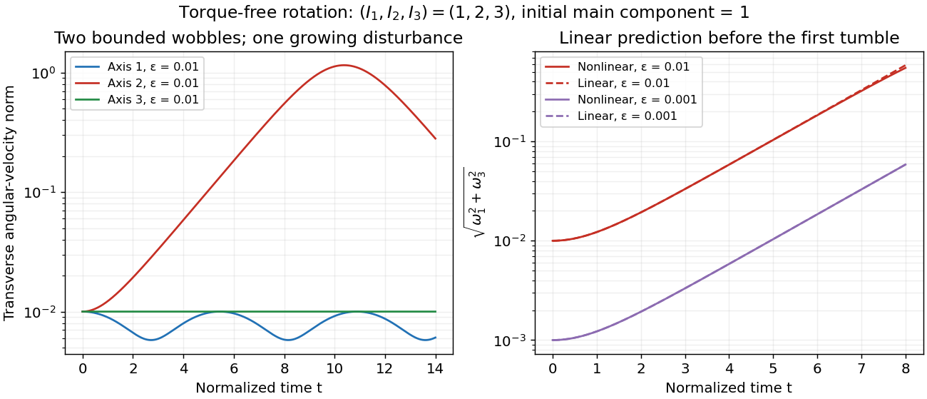
Small perturbations about the three principal axes
. Original Runge-Kutta method calculations for the normalized intermediate-axis model, with initial angular velocity , and . Left: transverse Euclidean norm relative to each initial principal axis. Right: full Euler equations for a torque-free rigid body compared with the displayed linearization, also using . Dashed curves are linear predictions. These are model curves, not measured throws. Details.
One-step method 2026-10-31
A one-step method approximates an ordinary differential equation using the current approximate solution and evaluations within the next step. The function is its increment function. A Runge-Kutta method may use several intermediate stages while remaining a one-step method: it does not require additional previous solution values as a linear multistep method does. Its consistency error is the exact-start update defect divided by .
Suppose an -stage Runge-Kutta method has order , an invertible matrix , and . Its stability function is . The adjugate matrix formula gives a rational function with denominator degree and numerator degree at most ; its zero limit at infinity lowers the latter degree to at most . The order of a numerical method gives , identifying the Padé approximant. Uniqueness follows because the cross-multiplied difference of two candidates has degree at most but a zero of order at least , so is identically zero. The A-stability of near-diagonal exponential Padé approximants then proves A-stability, and the zero limit proves L-stability. These conditions identify the stability function; they do not alone claim uniqueness of all entries of the Runge-Kutta method tableau.
Past exam of the mathematics course of the University of Cambridge 2001 iii Paper 57 1 Solution Created 2026-10-03 Updated 2026-10-14
Let be the coefficients of the -stage Runge-Kutta method. On the Dahlquist test equation , its stability function isBoth polynomials have degree at most , with denominator normalized to one at zero. Order implies . A rational function with these degree bounds and this accuracy is uniquely the diagonal Padé approximant . To see uniqueness directly, if and have the required accuracy, then is a polynomial of degree at most vanishing to order at least at zero, hence identically zero.
The diagonal exponential Padé approximant can be writtenUse the permitted Padé property that the zeros of lie strictly in the right half-plane and numerator and denominator are coprime. Thus has no poles in the closed left half-plane. Its real coefficients give , so . Also at infinity. Applying the maximum modulus principle on left half-disks and letting their radii increase proves for . There are no hidden stage poles there either: the irreducible Padé denominator has degree , exhausting the possible degree of , so the latter cannot contain an additional canceled factor. Every such maximal-order Runge-Kutta method is A-stable. This is maximal-order Runge-Kutta methods are A-stable; it does not assert L-stability, since the stability function does not tend to zero at infinity.
Past exam of the mathematics course of the University of Cambridge 2001 iii Paper 57 7 Solution Created 2026-10-03 Updated 2026-10-18
For an initial value problem, convergence of a numerical method means that on each fixed interval , the largest error at mesh points tends to zero as the step size tends to zero and the starting errors vanish. Order of a numerical method describes how rapidly an exact-start local defect decreases; stability of a numerical method controls propagation of that defect and of errors already present. These are related but different properties. A high-order expansion alone cannot ensure that accumulated error remains small.
For a one-step map , define the exact-start defect . Order means for sufficiently smooth solutions. The normalized local truncation error divides this defect by and is ; explicitly specifying the normalization prevents an apparent one-order discrepancy. Suppose the map satisfies the local Lipschitz boundFor the error recurrence isIteration, or the discrete Gronwall inequality, yields for . Stable propagation converts an order- local formula into global error , provided starting data are equally accurate. Consistency is the weaker requirement that the normalized local defect tend to zero.
For a linear multistep method, zero-stability concerns the recurrence at . Its roots must have modulus at most one, and unit-modulus roots must be simple. Roots outside the circle amplify errors exponentially in the number of steps; repeated unit roots introduce polynomial growth. The requirement is stronger than bounded propagation for one fixed number of steps: as on a fixed physical interval there are steps. Under the usual Lipschitz assumptions and consistent starting values, the Dahlquist equivalence theorem says consistency plus zero-stability is equivalent to convergence. Its sufficiency combines a bounded discrete recurrence propagator with the sum of local defects, while necessity follows by exciting an unstable homogeneous root or by observing the persistent error of an inconsistent formula.
For example, satisfies the first-order consistency identities, but its root polynomial is . For , a small starting error can excite a mode and destroy convergence as the number of steps increases. In contrast, simple parasitic unit roots such as the root minus one of a two-step centered method need not destroy zero-stability: they remain bounded, though they can create unwanted oscillations and affect practical behavior. Accurate starting procedures and suppression of accumulated parasitic error remain relevant.
Absolute stability asks a different question: for , does the discrete solution decay or stay bounded for a specified finite ? The Forward Euler method has and, for real , requires . It converges as , but a stiff decay mode can impose a severe practical step restriction unrelated to the accuracy needed for slowly varying components. The Backward Euler method has , hence is A-stable and L-stable. The trapezoidal rule has , is A-stable, but tends to minus one on a very stiff negative mode and can retain alternating transients rather than damping them rapidly.
Zero-stability therefore does not imply unrestricted absolute stability; the three-step family analyzed earlier in this paper is a particularly strong illustration. Conversely a stable large step need not be accurate. This distinction matters for a stiff equation. The Second Dahlquist barrier limits A-stable linear multistep methods to order at most two, whereas implicit Runge-Kutta methods can have much higher order and still be A-stable. That barrier concerns the specified method class, not every numerical time integrator.
Finally, the mathematical order depends on smoothness: nonsmooth solutions or forcing can lower observed rates. Roundoff, imperfect implicit solves and inaccurate derivative evaluations introduce additional defects. Smaller steps increase the number of such perturbations; truncation error alone does not describe arbitrarily fine computation. The useful organizing principle is consistency supplies vanishing defects, stability bounds their accumulation, convergence follows, and order quantifies its rate under the stated regularity and starting-error assumptions.
Past exam of the mathematics course of the University of Cambridge 2002 iii Paper 60 3 a Solution Created 2026-10-03 Updated 2026-10-14
Let be the vector of ones. For a general nonautonomous Runge-Kutta method the stages satisfy and the update is . Expansion at givesand thereforeThe exact solution is . Matching the independent terms gives the necessary and sufficient second-order conditions with independent Runge-Kutta abscissaeUnder the usual internally consistent Butcher tableau convention , this reduces to , , . If the abscissae are allowed to be independent of the row sums, is a sufficient simplifying convention rather than a logically necessary order-two condition.
Past exam of the mathematics course of the University of Cambridge 2003 iii Paper 67 1 a Solution Created 2026-10-03 Updated 2026-10-14
Introduce one stage with , and update . This is the implicit midpoint rule as a one-stage Runge-Kutta method, with Butcher tableauFor a smooth vector field, write . Expanding its stage equation giveswhich matches the exact Taylor expansion through degree two. The method therefore has order at least two. On the Dahlquist test equation , its stability function isThe third coefficient differs from the exponential's , so the order is exactly two.
There is no pole in , andThus throughout the closed left half-plane:This conclusion is A-stability, not strong damping of arbitrarily stiff modes: along the negative real axis.
Past exam of the mathematics course of the University of Cambridge 2004 iii Paper 69 1 a Solution Created 2026-10-03 Updated 2026-10-14
Apply the Runge-Kutta method to the Dahlquist test equation and put . Its stability function isSince is an invertible matrix, has polynomial degree . The adjugate matrix formula gives , but the additional condition givesso actually . The specified order of a numerical method implies near zero. Therefore the Padé identification of a Radau stability function makes the Padé approximant to the exponential function: its numerator and denominator have the required degrees, and its Taylor series agrees through degree .
In the permitted A-stability of near-diagonal exponential Padé approximants, take , . Then , so the scheme is A-stable. The same stability function also tends to zero at infinity, giving L-stability.