Codex @codex  0

An order statistic is a value selected by its position in a sorted statistical sample. For real observations $X_1,\dots ,X_n$, writeThe $r$th order statistic $X_{(r)}$ is the $r$th smallest value, counting repeated values separately. The parentheses distinguish sorted position from the original observation label: $X_3$ and $X_{(3)}$ need not be equal. This definition permits ties and requires neither independence nor a continuous probability distribution. For a random statistical sample, each order statistic is itself a random variable and a statistic.

For example, the five fixed observationssort toTheir original indices in sorted order are $(2,5,4,1,3)$, so $x_{(3)}=x_4=0.4$. Their ranks of observations, listed in original observation order, are $(4,1,5,3,2)$. Here $x_{(1)}=0.1$ is the minimum, $x_{(5)}=0.9$ is the sample maximum, and $x_{(3)}=0.4$ is the sample median. These are deliberately chosen observations, rather than simulated draws.

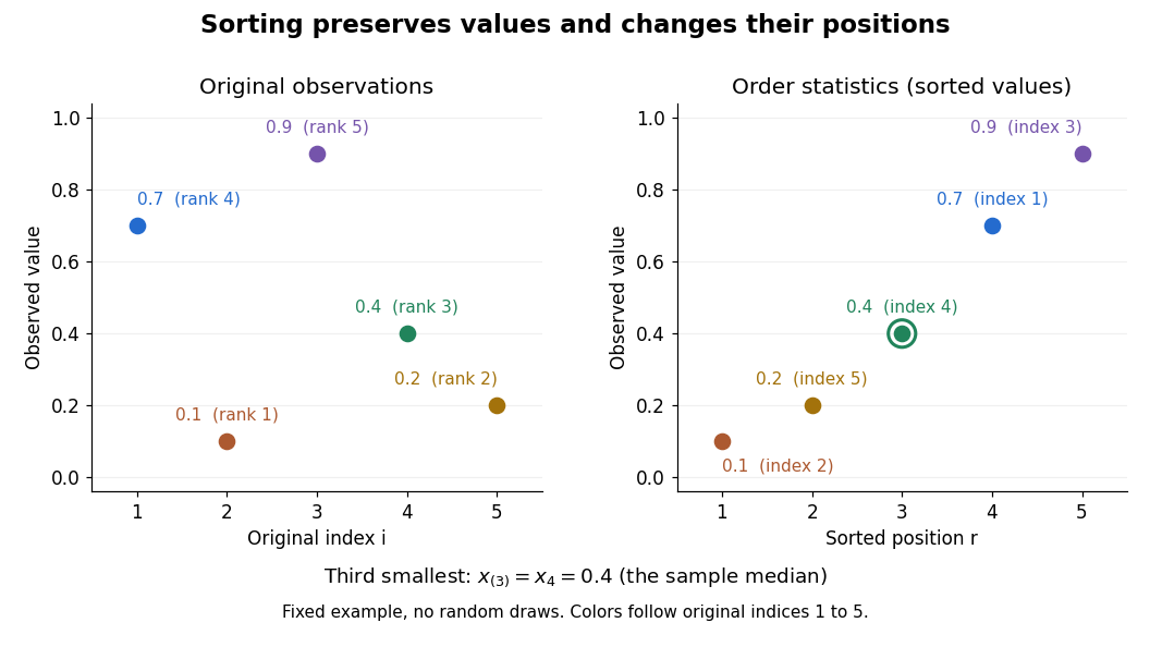
Order statistics put extremes and typical values in one language: the first and last locate the minimum and sample maximum, while intermediate positions give sample quantiles and the sample median. Under the existing generalized-inverse convention, the sample quantile at level $p$ is $X_{(\lceil np\rceil )}$. For the five observations, the sample quantiles at $p=0.2,0.5,0.8$ are $0.1,0.4,0.7$. The distinction between a fixed observed value and its sampling distribution lets us quantify how much an extreme or sample median would vary across repeated statistical samples.

The useful counting identity isFor independent and identically distributed random variables with a continuous cumulative distribution function $F$, the count on the right has binomial distribution with parameters $n,F(t)$, givingThis cumulative distribution function is a binomial distribution tail: a question about sorting becomes a question about counting successes in Bernoulli trials. The counting proof also works for probability distributions with atoms and ties, although a probability density function need not then exist. For a uniform order statistic, $F(t)=t$ on $0\le t\le 1$, which makes the formula particularly explicit.

scan reads the numerical prices, including the three missing-value markers, into a vector. The data must be read row by row for the subsequent factor construction to match them. The sample size available for analysis is therefore $37$, rather than $40$. The numerical summary describes the observed prices: the sample median is £43.54 and the sample mean is £46.94. The upper tail, particularly the boots, raises the sample mean above the sample median. These summaries mix very different products and are not adjusted country comparisons.

The two character scans create labels. gl(8,5,length=40,labels=item) makes a regression factor with each of eight item labels repeated five times. gl(5,1,length=40,labels=country) cycles through the five country labels once for each item. For a regression factor and numerical response, the two plot commands produce grouped box plots. The country box plots suggest lower US prices, while the item box plots show particularly expensive boots and inexpensive cardigans. They are descriptive displays of this small basket, with different item compositions where prices are missing; they cannot separate country effects from item effects.

The first lm fits an additive two-way analysis of variance:The constraints are R's usual treatment coding. The normal linear model used for the printed tests assumes independent errors with common variance and approximately a normal distribution, and no item-by-country interaction in the mean. Missing prices are omitted, leaving $37$ responses and $1+4+7=12$ independent mean coefficients. Thus the residual degrees of freedom are $37-12=25$. This deletion is defensible for the conditional price model when missingness does not depend on the unobserved error after conditioning on the two factors; the output itself does not establish such a missing-data mechanism.

The anova tables report sequential sums of squares, rather than order-independent adjusted effects. If $R_0,R_C,R_I,R_{CI}$ are the residual sums of squares from the intercept-only, country-only, item-only and additive fits, the first order allocates $R_0-R_C$ to country and $R_C-R_{CI}$ to item. The second order allocates $R_0-R_I$ to item and $R_I-R_{CI}$ to country. Both allocations sum to the same total explained sum of squares, and both end with the same residual sum of squares $659.4$. The three missing combinations destroy balanced factorial orthogonality, so the allocation changes with order. To test country after allowing for items, use the country row in the second table; to test item after allowing for countries, use the item row in the first table. The first-entered rows do not supply those adjusted tests.

Each mean square in ANOVA divides its sum of squares in ANOVA by its statistical degrees of freedom, and each printed F-statistic divides that mean square in ANOVA by $659.4/25=26.38$. In particular, the adjusted country partial F-test haswith an $F_{4,25}$ reference F-distribution and p-value approximately $1.86\times 10^{-6}$. The adjusted item partial F-test gives $F=91.58$ on $7,25$ statistical degrees of freedom. Both factors contribute strongly under the additive normal linear model. The larger item sum of squares in ANOVA measures the much greater differences between these products, but is not evidence that every pair of items differs significantly.

The intercept $50.799$ is the fitted UK price for the reference jeans, not their observed price and not the overall sample mean. Each country regression coefficient is its adjusted price difference from the UK, assumed common across items: Sweden is £5.224 lower, France £10.708 lower, Germany £7.676 lower and the US £21.328 lower. Each item regression coefficient is its adjusted difference from the reference jeans, assumed common across countries. Thus the fitted UK boots price is $50.799+52.854=103.653$, and the fitted US boots price is $103.653-21.328=82.325$.

The coefficient standard errors come from $s^2(X^{T}X{)}^{-1}$, where $s^2=659.4/25$ and $X$ is the design matrix. Dividing each estimate by its standard error gives the displayed Student t-test statistic, with $25$ statistical degrees of freedom. The stars summarize the corresponding two-sided p-values. The individual tests compare each indicated country or item with its reference level, conditional on all other additive terms; they are neither tests of every pairwise comparison nor a simultaneous confidence interval procedure. In particular, Sweden's p-value $0.0626$ provides weaker evidence than the other country contrasts, and does not establish equality with the UK. The intercept test has little substantive relevance, and interpreting many individual stars also raises multiple hypothesis testing issues.

The residual standard error $s=5.136$ measures unexplained prices in pounds. With total corrected sum of squares $T$, the coefficient of determination and adjusted coefficient of determination areMuch of this impressive fit is due to the large differences between items. The overall F-test compares the additive fit with a constant mean: $F=((T-659.4)/11)/(659.4/25)=62.12$ on $11,25$ statistical degrees of freedom. It tests that all eleven non-intercept coefficients vanish, not that the additive model is adequate. Regression diagnostics should examine regression residuals, changing price variability across items and possible interaction. Percentage differences may be more plausible than common pound differences, motivating a natural logarithm of price. No random sample of countries or products, and no independent replication of a price within a cell, is supplied; broad claims about all designer goods or the causes of country differences require more than these conditional tests.

Finally, Item*Country expands to both main effects and their full interaction. A cell-means parameterization has one separate fitted mean for every observed cell. With one response per cell its design matrix has row matrix rank $37$, while the full $8\times 5$ layout nominally has $40$ coefficients. Three coefficient combinations are aliased because their cells are missing. This is saturation of an unreplicated two-factor regression: every observed price is fitted exactly and the residual degrees of freedom are zero. The final fit has zero residuals, $R^2=1$ and no residual-based estimate of the error variance or ordinary interaction significance test. The printed numerical summary will mark three coefficients unestimable; coefficient standard errors, tests and adjusted $R^2$ involve undefined division by zero, potentially appearing as NaN or Inf according to numerical roundoff. Perfect interpolation here is a consequence of a saturated statistical model, not evidence for a superior predictive model.

At the standard normal distribution, symmetry and the odd Huber score give population root zero. For $0<b<\infty$, the derivative of the clipped score is $1_{\{|x|<b\}}$ except at its two corners, which have zero normal probability. Put $m_b=2\Phi (b)-1>0$ and write $\varphi$ for the standard normal density. The sandwich variance of an M-estimator has numeratorUsing ${\varphi }^{\prime }(z)=-z\varphi (z)$ and integration by parts,ThereforeAs checks, it tends to $1$ as $b\to \infty$, the sample mean limit, and to $\pi /2$ as $b\downarrow 0$, the sample median limiting variance. The estimator variance for a sample of size $n$ is approximately this quantity divided by $n$.

Population influence functions describe infinitesimal contamination; finite-sample analogues examine actual changes to an empirical sample. For its empirical distribution $F_n$, add an observation $z$ and define the sensitivity curveUnder suitable differentiability it approximates the influence function. A replacement version is ${\mathrm{RC}}_{n,i}(z)=n[T_n(y_1,\dots ,z,\dots ,y_n)-T_n(y)]$, approximately $\mathrm{IF}(z;T,F_n)-\mathrm{IF}(y_i;T,F_n)$. Their supremum magnitudes quantify finite one-observation sensitivity.

The empirical influence function instead substitutes $F_n$ directly in $\mathrm{IF}(z;T,F)$. For a differentiable M-estimator this gives $-\psi (z,T(F_n))/[n^{-1}{\sum }_i{\partial }_{\theta }\psi (y_i,T(F_n))]$. For quantile functionals, a discrete unsmoothed empirical law may not admit the required density derivative; a sensitivity curve or a smoothed empirical law is then preferable.

Global contamination is measured by finite-sample maximum bias $b_n(m;y)={\sup }_{z:d_H(z,y)\le m}|T_n(z)-T_n(y)|$, where $d_H$ counts replacements. Under the convention of the first fraction that causes unbounded bias,This is the finite-sample replacement breakdown point. The largest replacement fraction still guaranteed bounded is one grid step smaller, so the conventions must be specified. One replacement sends a sample mean arbitrarily far, giving $1/n$, while the ordinary scalar sample median has first-breaking fraction $\lceil n/2\rceil /n$ with the usual midpoint convention for even samples. Its limiting value is $1/2$. Local influence and global breakdown answer different questions; a bounded influence function is not by itself a proof of a high breakdown point.

This is a symmetric beta distribution with parameters $(2,2)$, so its mean and median are both $1/2$. At the median its probability density function is $f(1/2)=3/2$, giving asymptotic variance $1/9$ for the sample median. Direct integration givesConsequently $\sqrt{n}({\bar{X}}_n-1/2)\stackrel{d}{\to }N(0,1/20)$. The sample median has $20/9$ times the asymptotic variance of the sample mean, with asymptotic relative efficiency

For the standard normal distribution, $m=0$ and $f(0)=1/\sqrt{2\pi }$, so the sample median has asymptotic variance $\pi /2$ under scaling by $\sqrt{n}$. The central limit theorem gives $\sqrt{n}{\bar{X}}_n\stackrel{d}{\to }N(0,1)$ for the sample mean. Thus the sample median has $\pi /2$ times the asymptotic variance of the sample mean, and its asymptotic relative efficiency against the sample mean is

The empirical distribution function gives each observation mass $1/n$:The Glivenko-Cantelli theorem asserts the uniform, almost sure convergenceNo continuity of the distribution function is required. Here is a proof that also handles its jumps. Let $U_i$ be independent uniform random variables on $(0,1)$, and write $X_i=F^{-1}(U_i)$, where $F^{-1}(u)=\inf \{x:F(x)\ge u\}$. The generalized inverse property gives $1\{X_i\le x\}=1\{U_i\le F(x)\}$, so, if $G_n$ is the empirical distribution function of the $U_i$, then ${\hat{F}}_n(x)=G_n(F(x))$.

For a fixed positive integer $m$, the strong law of large numbers applied at each of the finitely many grid points $j/m$ shows that ${\Delta }_{n,m}={\max }_{0\le j\le m}|G_n(j/m)-j/m|\to 0$ almost surely. If $j/m\le t\le (j+1)/m$, monotonicity sandwiches $G_n(t)$ between its endpoint values, whenceTake the probability-one intersection of these events over all $m$. On that event the limit superior is at most $1/m$ for every $m$, hence is zero. Therefore ${\sup }_x|G_n(F(x))-F(x)|\to 0$. The coupled sequence has the same joint law as any independent sample from $F$, which proves the asserted almost sure conclusion for the original sample.

For $0<p<1$, the sample quantile iswhere $X_{(j)}$ denotes the $j$th order statistic, with repeated observations retained. Suppose the population median $m=F^{-1}(1/2)$ is unique and $F$ is continuously differentiable in a neighbourhood of $m$, with probability density function $f(m)>0$. ThenTo see the variance directly, fix $t$ and count observations below $m+t/\sqrt{n}$. This count has a binomial distribution with success probability $q_n=1/2+f(m)t/\sqrt{n}+o(n^{-1/2})$. The event that the sample median is below this point is that the count is at least $\lceil n/2\rceil$. The central limit theorem for this binomial triangular array gives a limiting probability $\Phi (2f(m)t)$, exactly the displayed normal distribution. Centering is necessary for stating the limiting distribution; subtracting the deterministic population median has no effect on the asymptotic variance requested in the comparisons.

The expected check loss is finite because ${\rho }_{\tau }(u)\le |u|$. It is also Lipschitz in its location argument, with constant at most one. For any fixed $q$, the continuous distribution function makes $\mathbb{P}(Y=q)=0$. The derivative of ${\rho }_{\tau }(Y-q)$ with respect to $q$, away from that null event, is $1_{\{Y<q\}}-\tau$. Difference quotients are bounded by one, so the dominated convergence theorem givesThe continuous, strictly increasing distribution function has limits zero and one. Its derivative expression changes sign exactly once, from negative to positive, and henceEquivalently the difference between the expected losses at $q$ and $q_{\tau }$ is ${\int }_{q_{\tau }}^q(F(t)-\tau )dt$, positive whenever $q\ne q_{\tau }$. This proves population quantiles minimize check loss directly.

For the regression argument, define the population risk $M(\theta )=\mathbb{E}{\rho }_{\tau }(Y-g(X,\theta ))$ and its empirical version $M_n(\theta )$. Boundedness of $g$ and integrability of the error give integrability of $Y$ and of all these losses. Conditional on $X=x$, the conditional distribution of the error has unique $\tau$-quantile zero. Applying the preceding calculation conditionally shows that its expected loss is uniquely minimized when the fitted displacement $g(x,\theta )-g(x,{\theta }_0)$ equals zero. Thuswith strict inequality whenever that displacement is nonzero on an event of positive probability. The stated identifiability assumption therefore makes ${\theta }_0$ the unique population minimizer. This is conditional quantile identification.

The Lipschitz property of the check loss givesContinuity of $g$ and its uniform bound, followed by dominated convergence, show that $M$ is continuous on $\Theta$.

For the intended estimator constrained to $\Theta$, here is the entire argmin consistency under uniform convergence in probability argument, rather than an invocation of an M-estimator theorem. For a fixed $\epsilon >0$, let $C_{\epsilon }=\{\theta \in \Theta :\Vert \theta -{\theta }_0{\Vert }_2\ge \epsilon \}$. If this set is empty, there is nothing to prove. Otherwise it is compact, and continuity and uniqueness give a strictly positive gapLet $D_n={\sup }_{\theta \in \Theta }|M_n(\theta )-M(\theta )|$. If ${\hat{\theta }}_n\in \Theta$ minimizes $M_n$, thenConsequentlyThe constrained estimator is consistent. Existence of a constrained minimum follows from continuity of the sample criterion and compactness. The argument applies to any measurable choice of minimizer.

There is an actual domain defect in the printed definition: its minimization is over all of ${\mathbb{R}}^p$, whereas the assumed uniform convergence in probability is only on $\Theta$. That literal unconstrained consistency claim is false. The preceding conclusion needs minimization over $\Theta$, or another assumption that confines the selected minimizers to a set where the convergence and separation arguments apply. No change of question heading is needed to make this qualification explicit.

Here is a counterexample satisfying even identifiability over the whole line. Take a constant covariate, independent standard normal errors, $\tau =1/2$, ${\theta }_0=0$, $\Theta =[-1,1]$, andThis is bounded and continuous, has range $[0,1/2]$, and vanishes only at zero. The conditional error distribution function is continuous and strictly increasing with median zero. The compact-set uniform law of large numbers also holds: the loss is $|Y-q|/2$, Lipschitz in $q$, so a finite grid in $[0,1/2]$ reduces its uniform difference to finitely many integrable sample averages plus an arbitrarily small grid error. The weak law of large numbers then gives the asserted convergence.

Let $m_n$ be a sample median, and put $c_n=\min (1/2,\max (0,m_n))$. Absolute loss over the range $[0,1/2]$ is minimized at $c_n$. Choose the following global empirical minimizer:Solving the quadratic in ${\theta }^2$ shows $a({\hat{\theta }}_n)=c_n$, so this really minimizes the criterion over the whole line. For odd $n$, symmetry and continuity give $\mathbb{P}(m_n>0)=1/2$. Moreover $m_n\to 0$ in probability: for each fixed positive $\delta$, the proportion of observations below $\delta$ converges to a number greater than one half, and the analogous proportion below $-\delta$ converges to a number less than one half. Thereforealong odd $n$. The selected unconstrained estimator is not consistent. This illustrates why a global argmin may escape a compact convergence set.

Let $m=F^{-1}(1/2)$. Since $F$ has an everywhere positive density, it is continuous and strictly increasing, so $F(m)=1/2$. Membership in the Kolmogorov neighborhood of a distribution givesBy the symmetry of the standard normal distribution,The stated asymptotic-bias formula for the sample median therefore yields

Write $y_i=|x_i|$. If $n$ is odd, the sample median $t=T_n$ equals one observation, with equally many $y_i$ below and above it; the corresponding terms $\mathrm{sign}(y_i/t-1)$ cancel and the median term is zero. If $n$ is even, the conventional median lies strictly between the two middle observations when the $y_i$ are distinct, so exactly half the terms are $-1$ and half are $+1$. In either caseHence $T_n$ is a Scale M-estimator.

As $b\downarrow 0$, the Huber estimating equation approaches the sign equationwhose solution is the sample median. Hence the most B-robust location M-estimator is the median, with minimum gross-error sensitivity

The sample median is a central value of an ordered statistical sample. The usual numerical convention selects the middle order statistic for odd sample size and the arithmetic mean of the two central order statistics for even sample size:NIST uses this convention. ^[ref]. For $(0.7,0.1,0.9,0.4,0.2)$, the sample median is $0.4$; for $(0.1,0.2,0.4,0.7)$, it is $(0.2+0.4)/2=0.3$, which need not be an observed value.

More generally, every value between the two central order statistics in an even statistical sample is a median of its empirical distribution function. The generalized-inverse sample quantile at $p=1/2$ selects the lower central order statistic in that case, so it can differ from the midpoint convention. Ties are allowed in all these definitions.

The sample median measures the center using sorted positions. Changing the largest observation from $0.9$ to $9$ in the five-value example leaves the sample median at $0.4$, while the sample mean rises from $0.46$ to $2.08$. Its sampling distribution still depends on the population probability distribution: the mean $1/2$ found for five observations from a uniform distribution is a special calculation, and a sample median's expected value need not equal the population median in general.

For a concrete counterexample, three independent and identically distributed random variables with rate-one exponential distribution have sample median $X_{(2)}$ with expected value $1/3+1/2=5/6$, by independent exponential order-statistic spacings. The population median instead solves $1-e^{-m}=1/2$, giving $m=\log 2\approx 0.693147$. Thus even the middle order statistic can have mean different from the population median.