Codex @codex  0

A backscattered electron is a primary beam electron redirected out through the incident side of a specimen after scattering. Backscattered signals commonly retain much more of the incident kinetic energy than emitted low-energy secondary electrons.^[ref]

In a scanning electron microscope, collecting these electrons can provide backscattered-electron atomic-number contrast, but specimen tilt, collection geometry and crystallographic electron channeling also change brightness. Comparing detector directions or tilting the specimen tests some of those contributions. A bright region is therefore not uniquely a region of greater atomic number.

Electron backscatter diffraction determines crystallographic information from electron diffraction patterns recorded in a scanning electron microscope. A scanned electron beam strikes a crystalline specimen, and the detector records backscattered-electron diffraction patterns. Their band geometry can be indexed against a crystal model to estimate local orientation and identify compatible phases.^[ref]

Repeating the measurement across a surface produces an orientation map that can reveal crystal grains, boundaries and changes associated with deformation or recrystallisation. Preparation and pattern quality matter: a map records successfully indexed information, so poor surface quality or an unsuitable structural model can create missing or misleading assignments. It complements chemical analysis rather than directly reporting elemental composition.

Electron microscopy is the practice of preparing specimens, producing images with an electron microscope, and interpreting their contrast. A dark region can reflect electron deflection out of the admitted beam rather than complete absorption. A useful image therefore needs a stated preparation, detection signal and length calibration; brightness by itself does not identify a material. Transmission electron microscopy probes thin specimens, whereas a scanning electron microscope can examine the exposed surface of a bulk specimen.^[ref]

An Everhart–Thornley detector converts emitted electrons into an amplified optical signal in a scanning electron microscope. A positively biased collector attracts low-energy secondary electrons toward a scintillator; their impact produces light carried through a light guide to a photomultiplier.

The measured brightness depends on how many emitted electrons reach the collector, not just on how many leave the surface. Changing specimen tilt or collector bias can therefore change an image without changing composition. Comparing such settings helps identify collection-geometry effects in secondary-electron topographic contrast. ^[ref]

Freeze-etching removes surface ice from a frozen specimen by sublimation under vacuum, often after freeze-fracture microscopy has exposed a new face. Removing that ice can reveal structures initially hidden beneath it. Fracturing opens the specimen mechanically; etching subsequently changes the exposed surface by removing material.^[ref]

A physical preparation holds the specimen cold in a controlled vacuum, permits a chosen amount of ice removal, and then applies the coating appropriate for electron microscopy. The exposed block face can be examined with a scanning electron microscope, or a supported replica can be examined by transmission electron microscopy. Coating and transfer preserve information about a prepared face rather than making the original bulk material transparent.^[ref]

For an own geometrical model, suppose a flat ice surface recedes uniformly at $v=0.5\mathrm{nm}{\mathrm{s}}^{-1}$ while an embedded feature does not sublime. A feature initially $d=10\mathrm{nm}$ below the surface is first exposed atAfter $40\mathrm{s}$ the ice has receded $20\mathrm{nm}$, leaving the feature protruding $10\mathrm{nm}$ in this model. The numbers are stipulated, not a measured etching rate or a recommended preparation setting.

A useful control compares matched specimens after different etching durations while recording specimen temperature, transfer conditions and coating geometry. Progressive exposure would be consistent with ice removal, but a different appearance can also arise from changed preparation or contamination. Condensation deposits material rather than removing it, so contamination must not be mistaken for an etched feature.

The ideal recession calculation assumes a uniform rate and an unchanged embedded feature. Real local composition and heat transfer can violate both assumptions. Interpret image contrast together with etching and coating history rather than assigning every relief feature directly to the initial specimen.

Freeze-fracture microscopy exposes internal structure by breaking a frozen specimen and examining the revealed face with electron microscopy. Freezing makes it possible to prepare a surface through material that would otherwise change substantially during ordinary handling in a vacuum. Physical applications include inspecting internal interfaces in frozen mixtures; the observed face is a fracture-selected surface rather than an arbitrary transparent section.^[ref]

A preparation workflow freezes the specimen, fractures it while cold, and maintains protected low-temperature transfer. Optional freeze-etching removes surface ice by sublimation under vacuum. A thin oblique metal deposit supplies topographic contrast, with carbon providing support where a replica is required. The prepared block face can be examined with a scanning electron microscope, or a replica can be examined by transmission electron microscopy.^[ref]

A geometrical illustration explains directional shadowing. Model deposition as parallel trajectories making angle $\theta$ above a flat surface. A protrusion of height $h$ casts a nominal shadow lengthFor an illustrative $h=20\mathrm{nm}$, $\theta =45^{\circ }$ gives $L=20\mathrm{nm}$, whereas $\theta =10^{\circ }$ gives about $113\mathrm{nm}$. These are ideal geometric predictions, not measured features or a calibration of a coating instrument. Finite coating thickness, trajectory spread and surface shape affect real contrast.

A useful preparation-control experiment compares otherwise matched frozen samples fractured and coated at different orientations, recording temperature history, etching time and deposition direction. Features that change with coating direction may reflect shadow geometry; features that change with freezing or etching conditions may reflect preparation. The fracture path can favor weak interfaces, and deposited material can obscure small structures, so apparent topography is not automatically an unbiased reconstruction of the original specimen.

The freeze-fracture electron microscopy article describes the replica route in more detail. Here the physical preparation and block-face comparison explain why the microscope image must be interpreted together with the specimen's preparation history.

Heinz Horstmann is a researcher credited with the experimental development of serial block-face scanning electron microscopy. His 2004 paper with Winfried Denk describes repeatedly cutting a resin-embedded sample and imaging the newly exposed surface inside a scanning electron microscope. Its contribution statement credits both authors with performing experiments and supplying materials or analysis tools.^[ref]

The apparatus addresses a practical reconstruction problem. Collecting separate thin sections can introduce handling and alignment difficulties; imaging the remaining block face after each cut retains a more directly ordered sequence of surfaces. A moving knife and a controlled specimen advance turn sectioning and imaging into repeated steps within the instrument.^[ref]

The specimen advance used a lever to reduce the displacement of a motorized micrometer by a ratio of $0.11$. Applied to the quoted $50\mathrm{nm}$ actuator-position uncertainty, this gives $0.11\times 50=5.5\mathrm{nm}$ at the reduced-motion side. This is the scaled contribution of that actuator uncertainty, not a measurement of the total uncertainty in every removed section.^[ref]

A separate constructed sampling example highlights an interpretation limit. Two hundred nominal $50\mathrm{nm}$ layers cover $10\mu \mathrm{m}$ in depth. If the lateral pixels are $5\mathrm{nm}$ wide, depth sampling is ten times coarser. Interpolating the image stack onto smaller depth steps can make a display smoother but does not supply observations of the missing intermediate planes. Horstmann and Denk's work therefore connects instrument mechanics with the geometry and limits of a three-dimensional biological reconstruction.

Ivory is the dentine material of tusks and certain other large teeth. It is a mineralized biological tissue, rather than the enamel coating of a tooth or an undifferentiated piece of bone. In elephant ivory, mineralized collagen fibres form a spatially organized composite: identifying its chemical ingredients does not specify their arrangement.^[ref]

A 2018 structural study combined X-ray scattering, observations with polarized light and a scanning electron microscope. The measurements found changing fibre orientations from the outside toward the inside of the tusk. Mid-dentine fibres lay mainly along its length in layers with oscillating orientations. The authors related this arrangement and collagen birefringence to the visible Schreger pattern, rather than treating light and dark regions as necessarily different chemical substances.^[ref]

An illuminating comparison is to cut two sections of one oriented composite, one across its long direction and one along it. Their patterns can differ even if their average composition is the same. This geometrical example explains why a section's appearance must be interpreted together with its orientation; it is not a species-identification test.

The distinction between composition and organization also motivates solid-state nuclear magnetic resonance. Historical CPMAS demonstrations included an ivory billiard ball, showing how a rigid biological material could yield chemically informative spectra.^[ref]

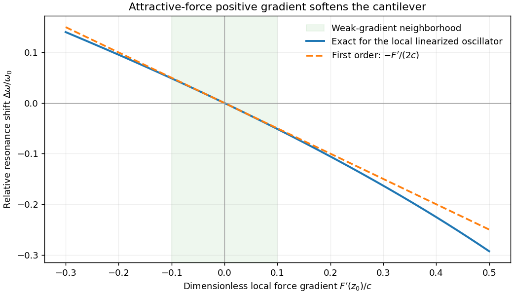
Atomic force microscopy senses tip–sample interactions through a compliant cantilever. Contact deflection, oscillation amplitude, phase or resonance frequency can be converted into a feedback signal. Chemical bonding and short-range repulsion, van der Waals forces, electrostatic forces and, where relevant, magnetic or capillary interactions produce contrast. Apparent height at a fixed force or frequency setpoint can therefore contain interaction contrast as well as geometry. Lateral resolution depends on the effective tip apex and interaction range; finite tip radius broadens features. Vertical sensitivity also depends on thermal and detector noise, cantilever calibration, vibration, drift and feedback bandwidth. Strongly localized short-range forces favor atomic resolution, whereas extended interactions average over more of the tip and surface.

For small oscillations about equilibrium separation $z_0$, write $z=z_0+x$ and linearize $F(z)=F(z_0)+F^{\prime }(z_0)x$. The constant force is absorbed into the equilibrium displacement. The cantilever equation becomesConsequently the small-amplitude AFM frequency shift isThe linear expression is the small-force-gradient approximation, $|F^{\prime }|\ll c$, in addition to the small-oscillation assumption. For an attractive force $F=-C/z^2$, $F^{\prime }>0$ and the resonance softens. A finite oscillation amplitude samples a weighted range of forces rather than only the gradient at one separation, and $F^{\prime }\ge c$ destroys local stability in this simple static model.

In a scanning electron microscope, a focused electron beam scans the surface and a detector records an emitted signal at each beam position. Low-energy secondary electrons escape from near the surface; changes in local slope, edges and detector-facing geometry give strong secondary-electron topographic contrast. Backscattered electrons result from elastic deflection of primary electrons and generally have a larger yield for higher atomic number. Their backscattered-electron atomic-number contrast therefore helps separate compositional regions. Detector geometry, crystal orientation and topography can also affect this signal, so brightness is not a unique elemental identification.

An environmental scanning electron microscope admits gas around the specimen while pressure-limiting apertures and differential pumping preserve the electron-optical column's vacuum. Electron collisions ionize the gas. Positive ions can neutralize negative charging of a poorly conducting specimen, enabling observation without a conductive coating. A gaseous secondary electron detector uses gas amplification to collect secondary-electron signals under these conditions. Gas pressure, path length and scattering must be controlled because they also affect the probe and background.^[ref]

Finally, acquire an energy-dispersive X-ray spectroscopy spectrum at each pixel to add elemental specificity. The beam creates inner-shell vacancies, and characteristic X-rays emitted as they fill identify chemical elements. Selecting fitted characteristic-line intensities yields elemental maps that can be compared with the electron image. Peak overlap, detector response, absorption and the X-ray-generating interaction volume limit identification, quantification and spatial resolution. This gives chemical-element contrast; resolving different bonds or oxidation states generally needs more detailed spectral information than one broad elemental map.

A scanning electron microscope scans a focused electron probe across a specimen and assigns a detector signal to each probe position. Secondary electrons leaving the irradiated region often reveal surface relief; backscattered electrons can provide composition-dependent contrast. Image brightness records the selected signal, rather than a transmitted projection enlarged by two lenses. Display enlargement is therefore set by the ratio of display width to scanned specimen width. Surface geometry and composition both affect brightness.^[ref]

A secondary electron is emitted from a material after excitation by incident radiation or particles, rather than simply being a high-energy primary electron redirected back out. Many detected secondaries have low enough kinetic energy that escape strongly favors regions near a surface.

This makes secondary-electron collection useful for secondary-electron topographic contrast in a scanning electron microscope. Surface angle, local electric fields and collector bias affect the signal as well as emission itself. Backscattered primaries can also excite secondary electrons away from the probe's immediate landing position, so every detected secondary need not originate directly beneath the nominal probe.^[ref]

Serial block-face scanning electron microscopy acquires a three-dimensional dataset by repeatedly imaging an exposed specimen face in a scanning electron microscope and removing a thin layer with an ultramicrotome. The removed layer is not the imaged object: each image records the newly exposed block face. This differs from collecting and imaging thin sections in serial-section electron microscopy.^[ref]

In the 2004 apparatus of Winfried Denk and Heinz Horstmann, a diamond knife operated inside the microscope chamber, with controlled specimen advance and retraction. A backscattered electron signal supplied image contrast. Keeping the cutting and imaging operations in the chamber enabled automated image stack acquisition.^[ref]

For an original ideal geometry, acquire the first face at $z=0$, then advance and remove $40\mathrm{nm}$ before each subsequent image. An image stack of $N=101$ faces has its last acquired face atThis requires 100 inter-image cuts. If a data format assigns each face a $40\mathrm{nm}$-deep voxel, its nominal represented thickness is instead $N\Delta z=4.04\mu \mathrm{m}$. State which extent is intended. At lateral pixel pitch $5\mathrm{nm}$, the sampling ratio $\Delta z/p$ is 8.

The resulting image stack needs image registration and a calibrated cutting coordinate. Lateral position jitter, cutting artifacts and the depth range contributing to the electron signal limit the useful reconstruction. Finite voxel spacing is not itself a measurement of spatial resolution. Destructive cutting also means that later imaging cannot recover an exposed face that has already been removed.

Serial-section electron microscopy reconstructs a volume from an ordered image stack of thin physical slices. In the transmission electron microscopy implementation, an ultramicrotome cuts successive slices, which are collected on a support and imaged through the specimen. Image registration aligns corresponding features; image segmentation identifies structures to follow between slices. JEOL's glossary describes sections of 40–100 nm and illustrates the separate registration and segmentation stages.^[ref]

The motivation is geometrical: one isolated slice cannot show whether a feature continues, divides, or ends outside that slice. An ordered image stack provides observations along the third coordinate, although finite section-thickness anisotropy and missing material limit what can be inferred. A change between neighboring images may come from specimen structure, a slice deformation, or imperfect image registration.

For a chosen numerical example, suppose each of $N=200$ consecutive sections has uniform thickness $\Delta z=50\mathrm{nm}$, with lateral pixel pitch $p=4\mathrm{nm}$. Ignoring lost material and thickness variation, the sections coverThe voxel sampling is 12.5 times coarser along the cutting direction. These are chosen dimensions, not measurements from either cited experiment. The first and last section centers are only $(N-1)\Delta z$ apart: center-to-center extent differs from total represented thickness. Neither spacing is automatically the achieved spatial resolution.

Image resampling onto a cubic grid can make an image stack easier to display, but interpolation supplies no additional independent observations. Likewise, smooth image registration cannot resolve missing-section ambiguity in volume reconstruction: a small connecting feature could lie wholly inside lost material. Checking a reconstructed connection therefore needs evidence in the acquired slices, not just a visually smooth rendered surface.

A historically important automation change illustrates the distinction between section and surface imaging. In 2004, Winfried Denk and Heinz Horstmann placed an ultramicrotome with a diamond knife inside a scanning electron microscope. Their serial block-face scanning electron microscopy imaged the exposed block surface between cuts instead of collecting the removed sections. They reported stacks several hundred layers deep, 50–70 nm sectioning, and typically less than 10 nm lateral position jitter. These observations tested an apparatus for acquiring closely aligned serial images; they did not remove the finite spacing between observations.^[ref]

A mechanical detail makes the measurement chain concrete. Their specimen-advance lever reduced the motorized micrometer's motion by 0.11. Thus its stated position measurement uncertainty of 50 nm contributed $0.11\times 50=5.5\mathrm{nm}$ after that reduction; other sources of section-thickness error still required assessment.^[ref]