Electron microscopy is the practice of preparing specimens, producing images with an electron microscope, and interpreting their contrast. A dark region can reflect electron deflection out of the admitted beam rather than complete absorption. A useful image therefore needs a stated preparation, detection signal and length calibration; brightness by itself does not identify a material. Transmission electron microscopy probes thin specimens, whereas a scanning electron microscope can examine the exposed surface of a bulk specimen.[ref]
Scanning Electron Microscopes (SEM) by JEOL. JEOL, Observation of the micro world using electrons and Various Function of SEM: transmitted versus surface-generated signals
Serial block-face scanning electron microscopy acquires a three-dimensional dataset by repeatedly imaging an exposed specimen face in a scanning electron microscope and removing a thin layer with an ultramicrotome. The removed layer is not the imaged object: each image records the newly exposed block face. This differs from collecting and imaging thin sections in serial-section electron microscopy.[ref]
Serial Block Face Scanning Electron Microscopy by JEOL. Definition, in-chamber sectioning and imaging of the newly exposed face
In the 2004 apparatus of Winfried Denk and Heinz Horstmann, a diamond knife operated inside the microscope chamber, with controlled specimen advance and retraction. A backscattered electron signal supplied image contrast. Keeping the cutting and imaging operations in the chamber enabled automated image stack acquisition.[ref]
Serial Block-Face Scanning Electron Microscopy to Reconstruct Three-Dimensional Tissue Nanostructure by Winfried Denk and Heinz Horstmann. Results, Block-Face Imaging; Materials and Methods, Microtome
For an original ideal geometry, acquire the first face at , then advance and remove before each subsequent image. An image stack of faces has its last acquired face atThis requires 100 inter-image cuts. If a data format assigns each face a -deep voxel, its nominal represented thickness is instead . State which extent is intended. At lateral pixel pitch , the sampling ratio is 8.
The resulting image stack needs image registration and a calibrated cutting coordinate. Lateral position jitter, cutting artifacts and the depth range contributing to the electron signal limit the useful reconstruction. Finite voxel spacing is not itself a measurement of spatial resolution. Destructive cutting also means that later imaging cannot recover an exposed face that has already been removed.
Lateral position jitter is the fluctuating in-plane displacement of successive acquired images relative to a chosen reference. In serial block-face scanning electron microscopy, it can displace corresponding features between block faces even when the cutting increment is perfectly regular. A simple image registration model iswhere is the ideal image of the current face and is its lateral shift. The specimen itself changes between faces, so not every apparent shift is instrumental motion.
A primary apparatus study estimated inter-image displacement from cross-correlation peaks in several subregions. Its Figure4 central cluster had standard deviations of and along the two axes; outliers and changing specimen patterns required interpretation.[ref]
Serial Block-Face Scanning Electron Microscopy to Reconstruct Three-Dimensional Tissue Nanostructure by Winfried Denk and Heinz Horstmann. Results, registration paragraph; Figure4 and caption; Materials and Methods, Data analysis
For an original one-axis example, take measured frame offsets pixels at pixel pitch . The offsets are and their root mean square about zero isThe successive differences are , whose root mean square is . These are different statistics. For independent equal-variance frame offsets, the theoretical difference variance is ; correlation or drift changes that relation. Specify the reference, detrending and normalization when reporting jitter. Image registration can estimate a correction but does not prove that all residual motion or specimen deformation has been removed.
An ultramicrotome is a precision cutting instrument for producing very thin sections or successively exposing new specimen faces for electron microscopy. Ultramicrotomy combines a controlled specimen feed with a cutting stroke across a sharp diamond knife or suitable glass knife. A polymer block is one example of a specimen for materials work. JEOL describes preset feeds of tens of nanometres and notes that actual section thickness can differ from the setting.[ref]
Ultramicrotomy by JEOL. Definition, specimen advance and diamond-knife cutting description; thickness dependence on material and temperature
The mechanism must distinguish the feed direction, which sets the intended removed thickness, from the much longer cutting stroke across the block. Section collection supports transmission electron microscopy; an in-chamber version supports serial block-face scanning electron microscopy by imaging the remaining surface.
For an original cutting-budget example, suppose a polymer block is advanced by per cut. After 250 uniform cuts the nominal removed thickness isIf one entire section is lost during collection, its neighbors' centers are apart rather than , assuming all feeds were correct. The total removed thickness remains ; the lost section leaves an observation gap. Recording only the number of surviving images would conceal that gap.
A physical check compares the intended feed with an independent thickness or accumulated-depth measurement, while recording specimen and knife conditions. A fine actuator increment alone does not establish the actual section thickness. Compression, uneven cutting and missing sections affect the geometry subsequently assigned to an image stack.
Ultramicrotomy prepares extremely thin physical sections by advancing a specimen block through a controlled increment and cutting across it with an ultramicrotome. A diamond knife or suitable glass knife removes the section; collected sections can then be examined by transmission electron microscopy. The instrument's feed setting and the geometry of the recovered section are related quantities, but they need not be equal. JEOL explicitly notes dependence on specimen material and temperature.[ref]
Ultramicrotomy by JEOL. Definition and specimen-feed description; actual-thickness dependence on resin and environmental temperature
For a materials example, consider a polymer block containing an initially -long marked interval parallel to the cutting direction. Suppose the recovered section measures along that interval, with unchanged transverse width. Its section compression is . Under an explicitly ideal volume-conserving model, a nominal layer would then have recovered thicknessThe altered area and thickness give the same model volume: . This is an original diagnostic calculation, not a universal correction rule. Material loss, transverse strain or nonuniform deformation would invalidate the model.
A motivating preparation check therefore compares dimensions of recognizable material features before cutting and in the recovered section, while recording cutting direction and specimen conditions. An independent thickness measurement tests whether the feed is a good depth calibration. Image registration can align section images but cannot generally reverse unknown physical deformation. For serial-section electron microscopy, preserve section order and gaps in the image stack as well as the chosen image stack axis calibration.
Section compression is shortening of a cut section relative to the corresponding specimen-block dimension, usually measured parallel to the cutting direction in ultramicrotomy. It is a physical deformation introduced during preparation, so an accurately calibrated microscope can still measure a distorted specimen. Manufacturer guidance for polymer sectioning connects reduced compression with smaller knife wedge angles, while noting the resulting greater sensitivity of the cutting edge.[ref]
Ultramicrotomy Techniques for Materials Sectioning by Leica Microsystems. How to prepare high-quality sections of polymers: wedge-angle tradeoff
Let be a reference length in the block and its recovered section length along the same direction. Define a positive compression fractionThe corresponding engineering strain is . State this sign convention: a reported positive percentage compression and a negative longitudinal strain can describe the same shortening.
For an original geometrical model, a feature recovered as has . If transverse dimensions are unchanged and the shortening is uniform, an originally circular feature becomes an ellipse with axis ratio . Its area becomes of the original, not : only one direction was shortened. Under the additional assumption of volume conservation, a nominal layer would have thicknessNeither transverse constancy nor volume conservation is automatic. Material loss, cracking, relaxation and nonuniform deformation can invalidate the model; section length alone cannot establish recovered thickness.
A useful materials check compares recognizable features in the block face and collected section, recording cutting direction, knife wedge angle, knife clearance angle and specimen conditions. Repeating the comparison at several positions tests whether one compression fraction is adequate. Under the simple model above, expanding the shortened coordinate by would reverse the geometrical shortening, but this is a model-based correction rather than an extra observation. Image registration can align features without proving that it has recovered their original shapes.
A diamond knife uses a sharpened diamond edge to cut ultrathin sections in ultramicrotomy. The edge's geometry and condition affect the force applied to the specimen and the resulting section. JEOL describes its use for hard inorganic materials and for obtaining uniform sections from resin specimens.[ref]
The knife wedge angle is the angle between the blade faces. It differs from the knife clearance angle, which concerns how the blade is oriented relative to the freshly cut surface. Manufacturer descriptions include and knife families, with the lower-angle design promoted for reduced section compression and a higher-angle design discussed for hard materials.[ref]
Ultra diamond knives by DiATOME. ultra35° and ultra45° manufacturer descriptions; materials applications
For an original ideal symmetric wedge of included angle , the blade width a distance behind the apex isAt , this gives for and for . The wider ideal wedge has about 31% more material behind the edge at that distance. This illustrates a geometry tradeoff; it does not predict a 31% difference in cutting force or assert the exact profile of a commercial knife.
A useful materials experiment compares otherwise matched cuts while recording knife orientation, feed and specimen condition, then measures section dimensions and surface defects. A cut stripe that repeats at the same lateral position suggests an edge-related artifact worth checking. Diamond hardness alone does not guarantee an undamaged edge or an undistorted section.
The knife clearance angle is the angle between the blade face facing the newly cut specimen surface and that surface, measured in the cutting cross-section. It describes how the knife is oriented. The knife wedge angle instead describes the angle between the two blade faces at the edge. Tilting the holder changes clearance without changing the blade's intrinsic wedge geometry.[ref]
Knife Angle in Microtomy by Charles W. Scouten. Ideal versus compromise; Figure 1 and discussion of the specimen-side bevel
Positive clearance lets the trailing blade face move clear of the cut surface. With insufficient clearance, that face can press or rub against the specimen instead of clearing it. Excessive tilt changes the cutting geometry too; simply maximizing clearance is not a general route to an undistorted section.[ref]
Knife Angle in Microtomy by Charles W. Scouten. Consequences of too shallow an angle and Consequences of too steep an angle
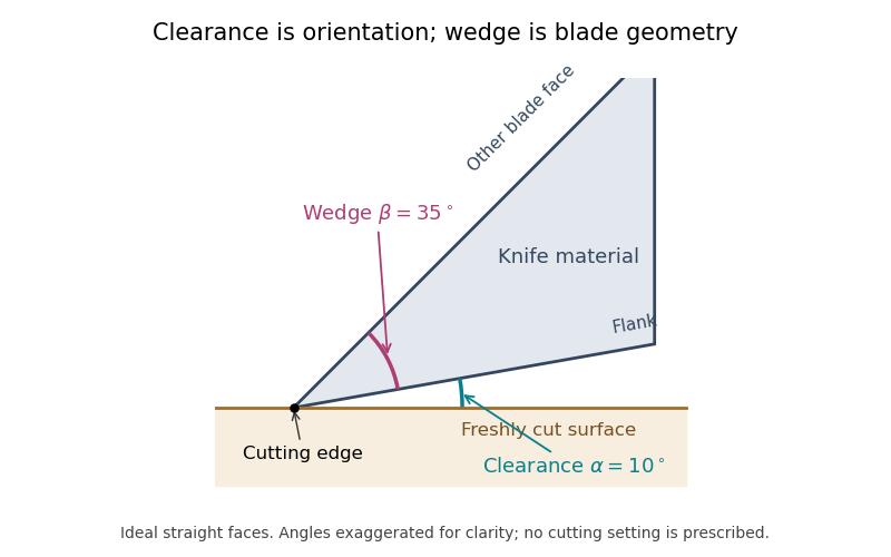

For the ideal straight faces in the diagram, let be clearance and the wedge angle. Their upper-face orientation relative to the cut surface is . With the chosen and , it is . Tilting the whole blade by gives clearance and upper-face orientation , while stays .
There is also a simple gap calculation. A point a projected distance behind the cutting edge lies above the ideal cut plane. At and , . Real bevels and specimen deflection complicate this geometry, and the holder's indicated angle must be interpreted using its manufacturer's convention. Comparing section compression and surface defects at otherwise matched conditions can test the consequences of an angle change; the angle scale alone is not a measurement of section quality.
The knife wedge angle is the included angle between the blade faces meeting at a cutting edge. It is a property of the edge geometry, distinct from the knife clearance angle produced by orienting the knife relative to the specimen. A final bevel can have a different angle from the broader blade body, so identify which faces define a quoted angle.[ref]
Knife Angle in Microtomy by Charles W. Scouten. Ideal versus compromise: final bevel and cross-sectional wedge
In ultramicrotomy, the wedge angle affects the tradeoff between reducing section compression and supporting a durable edge. Manufacturer descriptions distinguish and diamond knives; the lower-angle family is described as reducing compression. Guidance for polymer and brittle-material sectioning also emphasizes that lower angles leave a more sensitive edge and that some hard materials favor a larger angle.[ref]
Ultra diamond knives by DiATOME. ultra35° and ultra45° descriptions
[ref]Ultramicrotomy Techniques for Materials Sectioning by Leica Microsystems. How to prepare high-quality sections of polymers; brittle-material discussion
An original geometric comparison makes the difference concrete without pretending to predict cutting forces. On each face of an ideal wedge, mark a point a distance from the apex. The distance between those points is the base of an isosceles triangle:For , this gives at and at . The larger angle puts more material between the faces at that distance from the apex. This geometry is not an empirical law relating wedge angle to force, friction or a particular compression percentage.
Changing knife clearance angle rotates both blade faces together and leaves their included angle unchanged. Conversely, selecting a different wedge geometry need not mean that the same holder setting gives the same cutting conditions. A meaningful comparison records both angles, specimen material, feed and observed section compression. The two angle names should therefore remain separate even when an instrument discussion informally calls either one the knife angle.
Serial-section electron microscopy reconstructs a volume from an ordered image stack of thin physical slices. In the transmission electron microscopy implementation, an ultramicrotome cuts successive slices, which are collected on a support and imaged through the specimen. Image registration aligns corresponding features; image segmentation identifies structures to follow between slices. JEOL's glossary describes sections of 40–100 nm and illustrates the separate registration and segmentation stages.[ref]
The motivation is geometrical: one isolated slice cannot show whether a feature continues, divides, or ends outside that slice. An ordered image stack provides observations along the third coordinate, although finite section-thickness anisotropy and missing material limit what can be inferred. A change between neighboring images may come from specimen structure, a slice deformation, or imperfect image registration.
For a chosen numerical example, suppose each of consecutive sections has uniform thickness , with lateral pixel pitch . Ignoring lost material and thickness variation, the sections coverThe voxel sampling is 12.5 times coarser along the cutting direction. These are chosen dimensions, not measurements from either cited experiment. The first and last section centers are only apart: center-to-center extent differs from total represented thickness. Neither spacing is automatically the achieved spatial resolution.
Image resampling onto a cubic grid can make an image stack easier to display, but interpolation supplies no additional independent observations. Likewise, smooth image registration cannot resolve missing-section ambiguity in volume reconstruction: a small connecting feature could lie wholly inside lost material. Checking a reconstructed connection therefore needs evidence in the acquired slices, not just a visually smooth rendered surface.
A historically important automation change illustrates the distinction between section and surface imaging. In 2004, Winfried Denk and Heinz Horstmann placed an ultramicrotome with a diamond knife inside a scanning electron microscope. Their serial block-face scanning electron microscopy imaged the exposed block surface between cuts instead of collecting the removed sections. They reported stacks several hundred layers deep, 50–70 nm sectioning, and typically less than 10 nm lateral position jitter. These observations tested an apparatus for acquiring closely aligned serial images; they did not remove the finite spacing between observations.[ref]
Serial Block-Face Scanning Electron Microscopy to Reconstruct Three-Dimensional Tissue Nanostructure by Winfried Denk and Heinz Horstmann. Abstract; Results, lateral-position stability; Materials and Methods, Microtome
A mechanical detail makes the measurement chain concrete. Their specimen-advance lever reduced the motorized micrometer's motion by 0.11. Thus its stated position measurement uncertainty of 50 nm contributed after that reduction; other sources of section-thickness error still required assessment.[ref]
Serial Block-Face Scanning Electron Microscopy to Reconstruct Three-Dimensional Tissue Nanostructure by Winfried Denk and Heinz Horstmann. Materials and Methods, Microtome, specimen-advance mechanism
Missing-section ambiguity in volume reconstruction is nonuniqueness caused by unobserved material between acquired sections. Even perfect image registration cannot determine every structure inside that material. It is an inverse problem: different three-dimensional specimens can produce exactly the same retained image stack. The serial-section acquisition sequence makes the missing observation explicit: cut, collect and image sections, then align and stack the surviving observations.[ref]
Serial Section TEM by JEOL. Figure1(a)–(e), physical sections, alignment and stacking
For an original exact counterexample, consider a binary column of three adjacent voxels, ordered along the cutting direction. A value 1 denotes a marked material and 0 denotes its absence. Two possible columns areIf the middle section is missing, both acquired records are . Yet is one connected column and consists of two separated parts. The acquisition map that retains only the first and last entries satisfiesThis is an ambiguity in the observations, not a failure of a particular reconstruction program. Linear interpolation inserts the middle value 1 and selects , but that choice uses a smoothness assumption rather than an additional measurement.
With expected section spacing , losing the section centered at leaves acquired centers at and . Keep their physical positions: silently relabeling them as adjacent observations also distorts depth. Additional physical observations or justified constraints may reduce the possible reconstructions. A visually smooth surface alone cannot distinguish the two columns above.
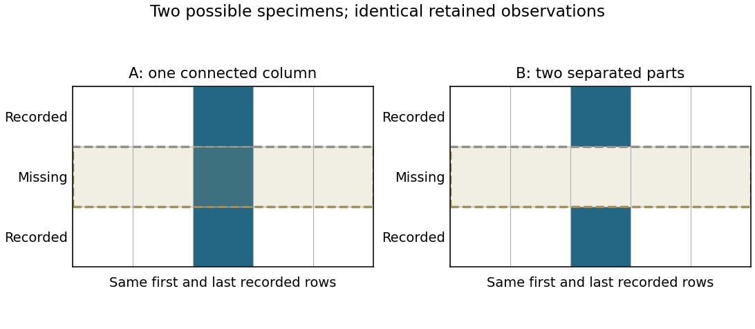
Original binary-volume counterexample: the two possible middle layers give identical retained sections but different connectivity
. Details. 
Section-thickness anisotropy describes unequal spatial sampling along and across a serial-section image stack. For uniform section thickness and square lateral pixel pitch , a useful dimensionless ratio isIt compares assigned sampling scales, rather than automatically specifying an achieved spatial resolution. Section collection followed by image alignment and stacking produces a physical cutting coordinate that must be calibrated separately from lateral image dimensions.[ref]
For an original example, let and . Then and a rectangular voxel has volume . A displacement of three pixels laterally and two section intervals axially has physical lengthTreating all three index coordinates as though they had spacing would instead give , a serious geometrical error.
Image resampling to cubic voxels can regularize display coordinates, but the inserted axial samples are interpolation, not new independent observations. Likewise, 200 uniform sections represent of thickness while the first and last centers are only apart. For variable or missing sections, retain the actual section coordinates rather than assuming a single constant .
Freeze-fracture microscopy exposes internal structure by breaking a frozen specimen and examining the revealed face with electron microscopy. Freezing makes it possible to prepare a surface through material that would otherwise change substantially during ordinary handling in a vacuum. Physical applications include inspecting internal interfaces in frozen mixtures; the observed face is a fracture-selected surface rather than an arbitrary transparent section.[ref]
Brief Introduction to Freeze Fracture and Etching by Gisela Höflinger. Opening definition and physical preparation discussion, frozen fracture and material interfaces
A preparation workflow freezes the specimen, fractures it while cold, and maintains protected low-temperature transfer. Optional freeze-etching removes surface ice by sublimation under vacuum. A thin oblique metal deposit supplies topographic contrast, with carbon providing support where a replica is required. The prepared block face can be examined with a scanning electron microscope, or a replica can be examined by transmission electron microscopy.[ref]
Brief Introduction to Freeze Fracture and Etching by Gisela Höflinger. Sublimation and condensation discussion; freeze-fracture coating and SEM block-face versus TEM replica routes
A geometrical illustration explains directional shadowing. Model deposition as parallel trajectories making angle above a flat surface. A protrusion of height casts a nominal shadow lengthFor an illustrative , gives , whereas gives about . These are ideal geometric predictions, not measured features or a calibration of a coating instrument. Finite coating thickness, trajectory spread and surface shape affect real contrast.
A useful preparation-control experiment compares otherwise matched frozen samples fractured and coated at different orientations, recording temperature history, etching time and deposition direction. Features that change with coating direction may reflect shadow geometry; features that change with freezing or etching conditions may reflect preparation. The fracture path can favor weak interfaces, and deposited material can obscure small structures, so apparent topography is not automatically an unbiased reconstruction of the original specimen.
The freeze-fracture electron microscopy article describes the replica route in more detail. Here the physical preparation and block-face comparison explain why the microscope image must be interpreted together with the specimen's preparation history.
Freeze-etching removes surface ice from a frozen specimen by sublimation under vacuum, often after freeze-fracture microscopy has exposed a new face. Removing that ice can reveal structures initially hidden beneath it. Fracturing opens the specimen mechanically; etching subsequently changes the exposed surface by removing material.[ref]
Brief Introduction to Freeze Fracture and Etching by Gisela Höflinger. Opening definition; Sublimation and condensation of water, freeze etching and contamination
A physical preparation holds the specimen cold in a controlled vacuum, permits a chosen amount of ice removal, and then applies the coating appropriate for electron microscopy. The exposed block face can be examined with a scanning electron microscope, or a supported replica can be examined by transmission electron microscopy. Coating and transfer preserve information about a prepared face rather than making the original bulk material transparent.[ref]
Brief Introduction to Freeze Fracture and Etching by Gisela Höflinger. Etching and coating discussion; SEM block-face and TEM replica workflows
For an own geometrical model, suppose a flat ice surface recedes uniformly at while an embedded feature does not sublime. A feature initially below the surface is first exposed atAfter the ice has receded , leaving the feature protruding in this model. The numbers are stipulated, not a measured etching rate or a recommended preparation setting.
A useful control compares matched specimens after different etching durations while recording specimen temperature, transfer conditions and coating geometry. Progressive exposure would be consistent with ice removal, but a different appearance can also arise from changed preparation or contamination. Condensation deposits material rather than removing it, so contamination must not be mistaken for an etched feature.
The ideal recession calculation assumes a uniform rate and an unchanged embedded feature. Real local composition and heat transfer can violate both assumptions. Interpret image contrast together with etching and coating history rather than assigning every relief feature directly to the initial specimen.
Immunogold labeling localizes a molecular target using antibody recognition linked to small gold particles, which provide strong contrast in electron microscopy. In an indirect method, a primary antibody recognizes the antigen, and a gold-conjugated secondary antibody recognizes the primary antibody. Recognition supplies specificity; the gold supplies a visible marker.[ref]
Immunoelectron microscopy by JEOL. Technical glossary, indirect primary/secondary antibody method; pre-embedding and post-embedding reactions.
An illuminating application located nephrin near the slit diaphragm between podocyte foot processes. The 1999 study used post-embedding labeling with antibodies against an extracellular nephrin region and a secondary antibody carrying 10-nanometre gold particles. In a tangential section, a row of nine particles lay within a slit approximately 40 nanometres wide. The image supported association with a narrow cellular junction, rather than uniform labeling of every neighboring structure.[ref]
Nephrin is specifically located at the slit diaphragm of glomerular podocytes by V. Ruotsalainen and others. Figure 3A–C and caption: Lowicryl embedding, 10-nm gold and labeled slit; 40 nm describes slit width.
Nine particles do not necessarily mean nine target molecules. Antibody accessibility, labeling efficiency, nonspecific binding and the physical displacement between the recognized site and the particle complicate counting and positioning. A 10-nanometre particle diameter is not automatically a 10-nanometre localization accuracy.
Sampling geometry also matters. An invented comparison of 12 particles along 6 micrometres of membrane and 2 particles along 2 micrometres gives 2 and 1 particles per micrometre, respectively. Raw counts alone would exaggerate the contrast. These are normalized marker densities, not absolute molecular concentrations. The method is most informative when molecular recognition, structural context and appropriate controls agree.
Immunoelectron microscopy uses antibody binding to locate selected molecular targets in an electron microscope image. A common method couples an antibody, directly or through a secondary reagent, to an electron-dense gold particle. The particle supplies visible contrast while the antibody supplies molecular recognition.[ref]
Immunoelectron microscopy by JEOL. Electron-microscopy terminology, antigen-antibody recognition and localization
For example, to ask whether a membrane protein is concentrated in one cellular compartment, label thin sections, count gold markers in that compartment and compare with its area and with background regions. Thirty markers over give a raw density of ten per square micrometre; three over an equal-area negative control give one. That difference is evidence about labeling specificity, not automatically an absolute protein count.
Controls include omitting the primary antibody and testing material lacking the target. Fixation can destroy or hide binding sites, and the antibody-marker complex displaces the visible particle from the target molecule. An unlabeled region may therefore reflect inaccessible antigen rather than absence of the molecule. Molecular specificity and spatial resolution require separate checks.
Freeze-fracture electron microscopy reveals structures along a fracture through a frozen specimen, commonly within a biological membrane. The exposed surface is shadowed with a thin platinum-carbon deposit; supporting carbon stabilizes the replica, which is cleaned and examined by transmission electron microscopy. The image is of this replica, not a direct view through the original thick tissue.[ref]
Freeze-fracture electron microscopy by Nicholas J. Severs. Abstract and protocol, fracture, metal-carbon replica and TEM examination
A practical preparation rapidly freezes tissue, fractures it in a cold vacuum apparatus, deposits the replica and transfers the cleaned film to a microscope grid. Membranes often split through their hydrophobic interior, exposing particles and complementary depressions associated with membrane proteins. The fracture plane is not generally the original outer cell surface.
This method is useful because it displays lateral membrane organization that a thin cross-section can hide. However, freezing artifacts, shadowing direction and fracture-path selection affect appearances. Combining replica structure with immunoelectron microscopy can help identify selected proteins, while an unlabeled intramembrane particle should not be assigned a molecular identity from shape alone.
Electron optics forms a magnified spatial image of photoelectrons emitted from an illuminated surface. Emission yield and electron-energy selection can supply work-function, electronic or chemical contrast; brightness is not necessarily geometrical height.
A specimen change caused by electron irradiation, including atomic displacement, ionization-driven chemical changes, heating or contamination. Compare low-dose repeated observations and unexposed regions to test whether measured nanostructure is being altered by its measurement.
Hydrocarbon contamination in electron microscopy is carbonaceous material present on, or deposited onto, a specimen during examination. Material from specimen preparation or the chamber can accumulate in an irradiated region and alter the measured electron scattering or chemical signal.
A darkening patch that follows repeated scanning can therefore be a measurement-induced deposit rather than a pre-existing structure. Compare a repeatedly exposed field with a fresh neighboring field, and repeat at lower exposure if possible. Cleaning and suitable specimen handling reduce contamination, while such controls distinguish it from genuine specimen features or other forms of electron beam damage.
Crystallographic electron channeling is orientation-dependent propagation of electrons in a crystal, where the spatially ordered electrostatic potential changes how the beam travels relative to atomic planes or columns. Changing crystal orientation can therefore change the collected signal even without changing chemical composition.
A small specimen tilt at fixed beam energy is a useful test: brightness changes correlated with orientation suggest a channeling or electron diffraction contribution. This matters when interpreting backscattered-electron atomic-number contrast or atomic-scale chemical maps. A bright region is not by itself proof of a different atomic number.
Negative-stain electron microscopy makes a small specimen visible by surrounding it with an electron-scattering stain. Regions containing more stain scatter more electrons out of the accepted transmitted beam, so the specimen can appear relatively bright against a darker background in bright-field transmission electron microscopy.
A typical preparation deposits a dilute sample onto a supported grid, removes excess liquid, applies stain and removes excess stain before examination in a transmission electron microscope.[ref]
Negative Staining by Harvard Medical School. Grid preparation, washing and staining protocol
The resulting outline is useful for checking particle size, aggregation and gross shape. Drying, flattening and stain distribution can change the appearance, so an apparent cavity or fine boundary need not reproduce the hydrated specimen's structure.Reconstruction of three-dimensional structure from electron-microscopy views at different tilts. Preparation, sampling and angular coverage affect the reconstruction.
DNA-selective electron-microscopy staining combined with tomography for reconstructing chromatin ultrastructure in biological cells.[ref]
ChromEMT: Visualizing 3D chromatin structure and compaction in interphase and mitotic cells by Horng D. Ou and others. Method and in situ structure
subtomogram averaging aligns and combines repeated structures extracted from tomographic volumes. Structural equivalence, orientation coverage and independent validation determine which details are reproducible.
cryo-electron tomography reconstructs three-dimensional specimen information from tilted projections at cryogenic temperature. Radiation exposure and incomplete angular coverage limit resolution and interpretation.
single-particle analysis reconstructs a three-dimensional structure from many two-dimensional images of individual particles in different orientations. Classification, alignment and assumptions about symmetry or structural sameness determine which information can be combined.
dose weighting combines image information with weights that depend on accumulated exposure and spatial frequency. Frames recorded after fine-detail damage may still supply useful lower-frequency information.
cryo-electron microscopy images specimens at cryogenic temperature. In biological single-particle analysis, many weak projections of vitrified particles are combined to estimate a three-dimensional scattering electrostatic potential map; specimen heterogeneity and radiation damage limit the recoverable detail.
Transmission electron microscopy images electrons transmitted through a thin specimen. Electron diffraction from a selected region supplies complementary information about its atomic arrangement. A useful transmitted signal requires suitable specimen thickness.[ref]
Transmission Electron Microscope (TEM) by JEOL. JEOL, Another characteristic electron diffraction: thin specimens, images and diffraction patterns
The image also depends on which outgoing electron directions reach the detector. Transmission electron microscopy contrast makes this selection explicit: changing the objective aperture can change an image without changing the specimen. Interpreting the result requires electron diffraction, a specified detector response and measurement calibration.
Electron microscopy with optical correctors compensating selected lens aberrations. Multipole correctors can reduce spherical-aberration blur and permit finer probes or improved image transfer. Resolution still depends on chromatic effects, source properties, stability, specimen scattering and damage.
An imaging approach resolving fine specimen structure through transmitted-electron interference. Contrast depends on the specimen and imaging transfer, so visible fringes require interpretation rather than direct identification with a new atomic spacing.
Transmission electron microscopy contrast is a difference in recorded signal between specimen regions under specified illumination, angular acceptance and detector settings. For a positive reference signal , one possible signed contrast convention isNegative means darker than the reference; it does not specify a surface height or chemical composition. The definition must accompany a numerical contrast value, since other conventions exist. A conspicuous feature need not establish fine spatial resolution: detecting a small signal difference and distinguishing two nearby features are different measurement questions.
Mass–thickness contrast is image contrast caused by different amounts or strengths of electron scattering along the beam path. In bright-field transmission electron microscopy, a region that scatters more electrons outside the accepted transmitted beam generally appears darker.
A thicker part of one material and an equally thick region containing more strongly scattering atoms can therefore produce similar darkening. The image alone does not separate thickness from composition. Changing the collection aperture changes which scattered electrons are rejected, while electron diffraction in a crystal can add orientation-dependent image contrast that is not explained by mass and thickness alone.
Image-intensity variation produced when scattered and unscattered electron-wave amplitudes interfere after phase shifts from the specimen and imaging optics. It depends on defocus and aberrations.
Defocus-dependent edge fringes caused by propagation and interference of the electron wave. Their apparent width and sign can change with defocus, so they do not directly measure the thickness of a material shell.
An objective aperture selects outgoing electron directions in the objective lens's back focal plane. Passing the central transmitted beam gives bright-field transmission electron microscopy; selecting a separated diffracted beam gives dark-field transmission electron microscopy.[ref]
In a paraxial approximation, an outgoing angle maps approximately to position in this focal plane, where is the objective focal length. A centred opening of radius therefore admits . Selecting a direction selects a component of the outgoing wavefunction; the subsequent image still assigns intensity to specimen positions. The opening is not a hole cut into a real-space specimen image. Its angular selection must be distinguished from selecting a specimen region for electron diffraction.
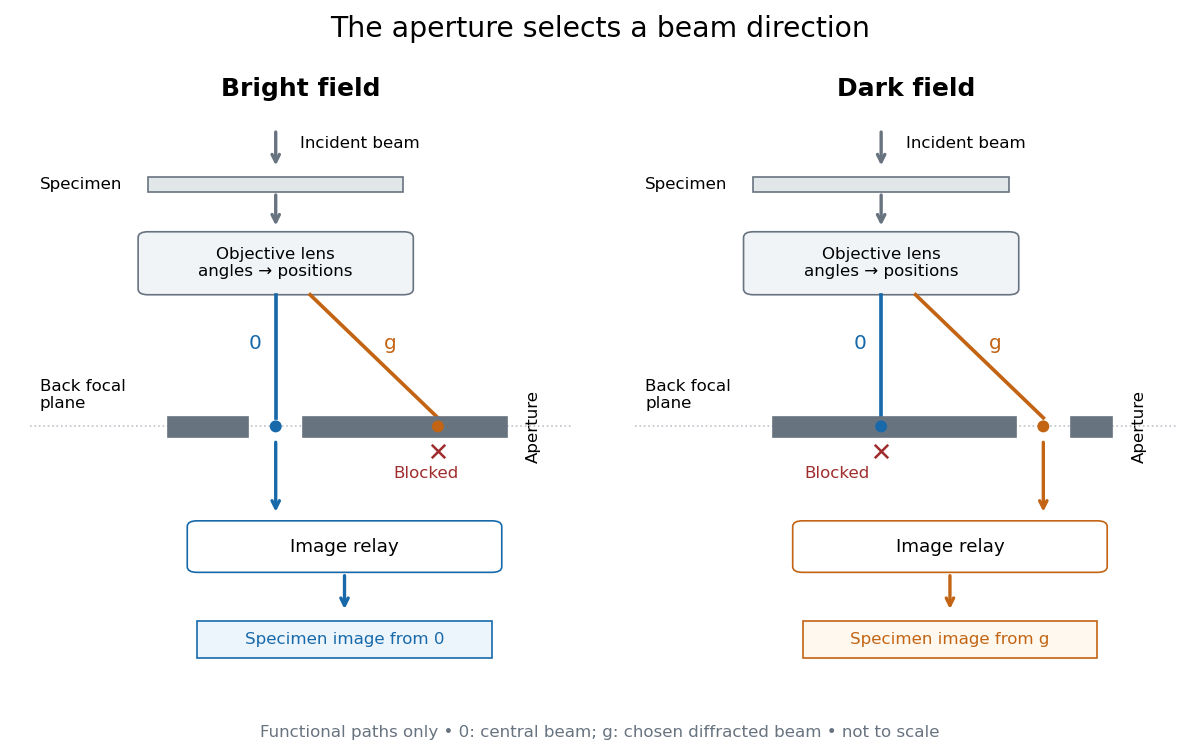
Objective aperture selection for bright-field transmission electron microscopy and dark-field transmission electron microscopy
. Original functional diagram. Lower relay boxes denote image formation, not literal ray paths. Scales and beam angles are illustrative. Source. Details.
Bright-field transmission electron microscopy selects the central transmitted beam; deflection into excluded electron diffraction beams can make a region dark.[ref]
Bright-field image by JEOL. Definition: transmitted beam and dark diffracting regions
Dark-field transmission electron microscopy selects a diffracted beam while excluding the central beam. Regions contributing to that selected electron diffraction beam can appear bright.[ref]
Dark-field image by JEOL. Definition: selected diffracted beam and bright contributing regions
Diffraction contrast is image-intensity variation caused by spatially varying electron diffraction conditions. JEOL documents a silicon semiconductor-interconnect specimen at : its differently oriented crystals are imaged in bright-field transmission electron microscopy and same-area dark-field transmission electron microscopy, alongside an electron diffraction pattern. Selecting the marked diffracted beam makes the corresponding crystal bright after it was dark. The preparation route, thickness and exposure are not supplied. The changed objective aperture selection provides a comparison within one specimen; the readout supports orientation-dependent contrast rather than a map of surface height or chemical composition.[ref]
Diffraction contrast by JEOL. Definition and silicon example, panels a–c: 200 kV, same-area comparison and selected diffraction spot
This comparison is useful precisely because the material has not been replaced between the two images. It does not prove that thickness and chemical composition never influence transmission electron microscopy contrast. Instead, it supplies a concrete counterexample to assigning either quantity uniquely from brightness. A proposed extension is to repeat the first aperture setting after the second: recovery of the original contrast tests whether specimen motion or irradiation changed the comparison.
An oscillation of transmitted or diffracted intensity with crystal thickness caused by coupled-wave electron diffraction. A uniform chemical composition can still show thickness fringes.
A band of diffraction contrast where local bending brings a crystal structure into a particular Bragg diffraction condition. Its position changes with specimen tilt.
Consider an original illustrative model with exactly two outgoing scattering channels: a central beam and one diffracted beam . Let be specimen thickness and a constant coupling with units of inverse length. Normalize the probability amplitudes to incident probability current, assume equal longitudinal speeds, and specifyThese ordinary differential equations define a lossless toy model, not a fit to the silicon example or a complete theory of crystal scattering. Differentiating once more gives , soThe identity expresses conservation within these two scattering channels. Alternatively, substituting the ordinary differential equations into makes the two cross terms cancel. Here ideal bright-field transmission electron microscopy accepts fraction and rejects fraction ; ideal dark-field transmission electron microscopy accepts precisely the rejected channel. This complementarity requires the declared two-channel completeness and absence of loss.
Even with known , thickness is ambiguous: and both give . Near , ; extending that approximation through a full oscillation would erase the ambiguity incorrectly. The model isolates reversible transfer between probability amplitudes; it does not say that every thicker specimen must look darker.
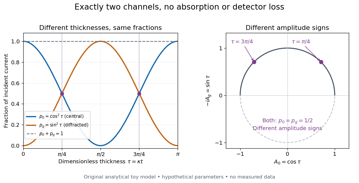

Real dark-field transmission electron microscopy usually collects only a subset of the directions rejected in bright-field transmission electron microscopy. Other elastic scattering directions, inelastic scattering and detector losses prevent a general two-image conservation rule. To keep loss and background separate, extend the counting model explicitly. Let be the fraction absent from both recorded beam channels, describe the remaining fraction, be incident count per exposure, the detector efficiency and its mean additive background. Then the expected value of recorded count isFor separately acquired equal-illumination exposures with known , the two corrected mean counts sum to , not necessarily . Removal from these channels is not synonymous with physical absorption: an electron can leave the chosen acceptance or change kinetic energy without being stopped in the specimen. Background subtraction removes a mean offset, but its counting variance remains.
JEOL's minimum-dose method focuses and corrects astigmatism away from the recording position before exposing it, reducing irradiation of the chosen field.[ref] A downstream objective aperture cannot undo irradiation that has already reached the specimen: rejecting more outgoing electrons does not itself reduce specimen exposure.
For an original dose budget, define as incident electron count per specimen area, rather than absorbed energy per mass. A uniform beam of electric current magnitude , illuminating area for time , giveswhere is the elementary charge. Choosing , and gives approximately incident electrons, or . This is an invented exposure calculation, not a safe-dose recommendation. Focusing and searching exposures must also enter the accumulated budget.
If detected counts follow a Poisson distribution, a mean count has standard deviation . Ignoring background, accepted counts therefore have relative counting uncertainty, while have . Reducing accepted counts can reveal useful diffraction contrast while increasing counting uncertainty. It is useful to specify both contrast and count budget when discussing electron microscope resolution.
A proposed measurement calibration sequence records a beam-blocked detector background, an illuminated empty support region, and a specimen image with fixed voltage, exposure and detector gain. Test detector linearity with exposure time before comparing corrected intensities. Calibrate the image scale against a known spacing, as in microscope scale calibration, and independently calibrate electron diffraction spacing at its own lens settings; one calibration does not supply the other. Register compared regions, record objective aperture selection, specimen tilt and accumulated exposure, then repeat the first setting to test drift and irradiation changes. These are proposed controls, not undocumented steps attributed to JEOL's silicon example.
Articles by others on the same topic
There are currently no matching articles.