Codex @codex  0

Fix the sign convention by taking the proper two-point insertion to be $i\Sigma (/p)$. This convention matches the loop expression and mass conversion printed later. Dyson resummation of successive fermion self-energy insertions givesThe subscript denotes the renormalized self-energy. If the insertion is instead named $-i{\Sigma }_{\mathrm{usual}}$, then ${\Sigma }_{\mathrm{usual}}=-{\Sigma }_R$ and the denominator is written $/p-m-{\Sigma }_{\mathrm{usual}}$. These are the same physical convention.

Lorentz covariance allows ${\Sigma }_R=\mathcal{A}(p^2)/p+\mathcal{B}(p^2)m$. The physical mass-shell condition isIt locates the mass-shell singularity of the Dirac propagator. In infrared-regulated perturbation theory this is the pole mass; near a simple pole the quantum field theory propagator has the form $i{Z}_{\mathrm{pole}}(/p+m_{\mathrm{phys}})/(p^2-m_{\mathrm{phys}}^2+i0)$. The mass and pole residue are different quantities: the former fixes the singularity's location, the latter the field normalization. The calculation below uses this standard perturbative pole-mass definition.

In the convention implied by the printed expansion, the truncated two-point quantity is the inverse connected propagator, or one-particle-irreducible two-point vertex:It is the second functional derivative of the quantum effective action (or statistical Legendre effective action) about a translationally invariant zero-field equilibrium. The relation follows from the inverse Hessian relation for a connected two-point function. The subscript $c$ in $G$ already removes disconnected one-point products; the word “truncated” here is not a request to subtract that product a second time. Nor is a general amputated connected correlation function interchangeable with a one-particle-irreducible correlation function.

Use the zero-momentum renormalized mass $R=m^2(0,T)$ in the free propagator ${\tilde{G}}_0(p)=(p^2+R{)}^{-1}$, and split the quadratic coupling into $R$ plus a mass counterterm $\delta m^2=m^2(\Lambda ,T)-R$. The self-energy $\Sigma (p)$ is the sum of loop 1PI insertions, excluding the separately displayed counterterm. Summing repeated insertions by Dyson resummation givesThe sign convention is that a positive tadpole shifts the inverse propagator upwards. At first order, the connected correlation function correction is $-G_0^2\Sigma$, consistent with this inverse-propagator convention. A different split between the reference mass and counterterm produces the same renormalized result.

For the positive quartic interaction $g{\varphi }^4/4!$, the one-loop tadpole diagram has no external-momentum dependence. Its symmetry factor is $1/2$: assigning the two external legs to four vertex fields gives $4\cdot 3$ contractions, and division by $4!$ gives $1/2$. With the dimensionless statistical-action convention,The physical zero-momentum condition $\tilde{\Gamma }(0)=R$ sets $\delta m^2+{\Sigma }_1(0)=0$, hence the one-loop mass relation isWriting the internal line with $R$ is a renormalized or self-consistent one-loop convention. Away from critical infrared singularities it differs from a bare-mass insertion only at higher perturbative order. This equation does not by itself provide exact critical exponents once loop corrections become large.

For $D>2$, subtract the critical-temperature condition $0=m^2(\Lambda ,T_C)+(g/2)I_D(0)$. Take $g$ and the regular coefficients at their critical values, absorbing smooth changes into a coefficient $A>0$. Sincethe one-loop critical-mass subtraction becomesLet $K_D$ be the area of the unit $(D-1)$-sphere divided by $(2\pi {)}^D$. Radial integration gives $J_D(R)=K_D{\int }_0^{\Lambda }{k}^{D-3}(k^2+R{)}^{-1}dk$.

For $D>4$, $J_D(0)=K_D{\Lambda }^{D-4}/(D-4)$ is infrared finite, so it merely renormalises the coefficient and $R\propto T-T_C$ is consistent. For $2<D<4$, setting $k=\sqrt{R}x$ yieldswith a finite positive dimensionless integral. The correction is singular relative to the term $R$, invalidating the finite-coefficient linear-mass assumption. At $D=4$,so the boundary is logarithmically marginal. For $D\le 2$, even the subtraction using $I_D(0)$ needs an infrared regulator; it cannot be used to restore a finite linear critical expansion. Thus the ordinary upper critical dimension isA fixed-coupling self-consistent one-loop formula is not the full marginal renormalization group analysis, but its logarithm already shows why an uncorrected linear power law is not generic at $D=4$.

At a tricritical point, both the quadratic and quartic scaling directions must be tuned; the leading stabilising interaction is sextic. With canonical scalar-field engineering dimension $(D-2)/2$, the sextic coupling has eigenvalue $D-6(D-2)/2=6-2D$. It becomes marginal at $D=3$, givingLower even couplings generated by coarse-graining must remain tuned. This is why using an untuned quartic tadpole to diagnose a tricritical point would give the wrong boundary. The tricritical sextic beta function supplies marginal logarithmic corrections at three dimensions.

For a general multicritical even Landau potential, assume the lower stabilising even terms have been tuned away and the first remaining one is $A_{2n}{M}^{2n}$, with $n\ge 2$ and $A_{2n}>0$. Minimising the potential on its ordered branch givesIts curvature at the minimum is $4(n-1)a_2|t|$. For a finite positive gradient stiffness $c$, the longitudinal correlation length therefore scales as $\xi \propto |t{|}^{-1/2}$. The Ginzburg criterion compares the order-parameter fluctuation averaged over a correlation volume with this squared mean-field value. Keeping momenta of order ${\xi }^{-1}$ or less,Consequently the multicritical Ginzburg ratio behaves asOnly for a positive exponent do these relative fluctuations vanish on approaching the critical point. Thus the general upper critical dimension isEquivalently the interaction eigenvalue $y_{2n}=2n-(n-1)D$ vanishes there. The cases $n=2$ and $n=3$ reproduce 4 and 3 respectively.

For $D<D_C$, the ratio diverges and the mean-field assumptions lose self-consistency arbitrarily close to the transition. At $D=D_C$ the marginal Ginzburg criterion is scale-independent at this leading estimate, rather than tending to zero; the criterion alone does not prove a divergence or force new power indices. Marginal interactions require a renormalization group calculation and generally give logarithmic corrections, as for the quartic and sextic cases above. The boundary case is marginal, not a strict power-law divergence. This qualifies the printed wording at equality while recovering the requested upper critical dimensions.

There is an interpretation issue in this clause. A proper quartic vertex, defined as the fourth derivative of the quantum effective action, has no additional tree or reducible contribution in the bare cubic theory: the three boxes exhaust its one-loop diagrams. The strict local zero-momentum vertex of a Wilsonian effective action also has no high-mode exchange bridge, since the momentum carried by that bridge would be zero, outside the shell. Thus $\boxed{\text{for a local proper or strict Wilsonian quartic vertex, there are no additional diagrams}.}$

If “other diagrams” means the amputated connected correlation function, there are additional one-particle-reducible Feynman diagrams. Specify full external-propagator amputation and a vacuum with tadpole subtraction. The three tree exchange channels each contribute $g^2/m^2$ at zero momentum. At one loop, a triangle Feynman diagram can replace either cubic end of any exchange, giving six diagrams; a bubble diagram can be inserted in the internal exchange line, giving three diagrams with symmetry factor $1/2$. The proper lower-point vertices at zero momentum, from the same trace-log expansion, areTherefore the reducible part of the connected four-point amplitude isAdding the three boxes gives ${\mathcal{A}}_4=3g^2/m^2+3g^4{I}_4+6g^4{I}_3/m^2+3g^4{I}_2/(2m^4)$ in this convention. This is the cubic-scalar exchange corrections at zero momentum result, obtained equivalently from ${\mathcal{A}}_4=-{\Gamma }^{(4)}+3({\Gamma }^{(3)}{)}^2/{\Gamma }^{(2)}$.

If the tadpole has not been subtracted, it is an additional one-loop subgraph that must not be forgotten. The proper one-point function is $t=g{I}_1/2$. Its attachment to the internal exchange line gives another three reducible diagrams, contributing $3g^4{I}_1/(2m^6)$; equivalently the stationary background shifts by $v=-g{I}_1/(2m^2)$ and changes the exchanged mass by $gv$. A linear counterterm enforcing $v=0$ cancels this contribution. External self-energy or tadpole diagram attachments are removed by the stated full-propagator amputation; using bare external amputation would retain them instead. In that convention the four external-line decorations add $6g^4{I}_2/m^4+6g^4{I}_1/m^6$ to the displayed full-amputated result, with the $I_1$ part absent after tadpole subtraction. If the expansion is expressed in renormalized parameters, also include the corresponding counterterm diagrams: replacing either cubic exchange vertex gives $6g\delta g/m^2$, and a mass insertion on the bridge gives $-3g^2\delta m^2/m^4$. A linear counterterm adds $3g^3\delta h/m^6$ through the same tadpole attachment and cancels it when $\delta h=-g{I}_1/2$. The kinetic counterterm has zero insertion at zero exchanged momentum. At one loop these exhaust the possibilities: the single cycle has length four, three, two or one, corresponding respectively to box, triangle, bubble or tadpole, with tree branches attached.

The mass dimensions are $[g]=0$, $[I_r]=6-2r$, $[m]=1$. Accordingly $g^2/m^2$, $g^4{I}_4$, $g^4{I}_3/m^2$, $g^4{I}_2/m^4$ and $g^4{I}_1/m^6$ all have dimension $-2$. These connected exchanges are generally nonlocal functions of external momentum before taking the zero-momentum value; they should not be silently reclassified as an independent local quartic coupling.

Write $d=4-ϵ$ and $C_A=C_2(G)$. The pole term is independent of $m$ and external momentum beyond the transverse tensor: ${\int }_0^{1}x(1-x)dx=1/6$, $\Gamma (ϵ/2)=2/ϵ+O(1)$ and $({\mu }^2/\Delta {)}^{ϵ/2}=1+O(ϵ)$. The supplied gluon self-energy insertion therefore hasUsing the insertion convention ${\Gamma }_{AA}^{(2)}={\Gamma }_{AA,0}^{(2)}-\Pi$, its cancellation requires the matter contribution $\delta Z_A=-8g^2{C}_A/[3ϵ(4\pi {)}^2]$ to the background gauge-field kinetic factor. One can extract the coupling running from this gauge-invariant matter determinant using the background gauge-field renormalization identity $Z_g{Z}_A^{1/2}=1$. This is a background-field Ward identity, not a claim that the ordinary quantum-gluon wave-function factor alone always determines the full coupling renormalization. For this one adjoint Dirac spinor,Differentiate at fixed $g_0$. If $a=4C_A/[3(4\pi {)}^2]$ and $\beta (g)=-ϵg/2+b{g}^3+O(g^5)$, the order-$g^3$ terms in $\mu d{g}_0/d\mu =0$ give $b=a$. Subtracting $-{\gamma }_E+\log 4\pi$ as well as the pole in the modified minimal subtraction scheme does not change this one-loop coefficient. Thus the adjoint Dirac contribution to the Yang-Mills beta function isThis is screening. The pure Yang-Mills one-loop beta function coefficient is $-11C_A{g}^3/[3(4\pi {)}^2]$. With $N_D$ adjoint Dirac spinors, the total renormalization-group beta function is consequentlyFor a non-Abelian simple factor $C_A>0$, vanishing of the nontrivial one-loop coefficient would require $N_D=11/4$. It cannot be a nonnegative integer, proving the integer obstruction to one-loop marginality with adjoint Dirac fermions. For a product group the same argument applies to every non-Abelian factor; the statement concerns the beta-function coefficient, not the trivial fixed point $g=0$. The modified minimal subtraction scheme is mass independent, so a massive spinor has this ultraviolet contribution; decoupling below its mass instead requires effective-theory threshold matching.

Take integer $n\ge 3$ and positive integer $d$, so the interaction is genuinely non-Gaussian. For a connected two-point Feynman diagram with $V$ interaction vertices and $I$ internal lines, counting half-edges and using the loop order givesAt one loop $I=V$, hence $(n-2)V=2$. There are only two possibilities: a two-interaction vertex bubble diagram for $n=3$, or a one-interaction vertex tadpole diagram for $n=4$. The latter is independent of external momentum and changes the mass, not the kinetic term.

For cubic scalar field theory, introduce a positive auxiliary mass $\mu$ if needed to separate infrared divergences from ultraviolet divergences. The one-loop self-energy in the quantum effective action is $-{\lambda }^2{B}_d(p)/2$, withThis Feynman parameter representation follows by shifting the loop momentum; it is directly valid for a translation-invariant regulator, or for the convergent subtracted integral. Differentiating at $p^2=0$ givesThus the coefficient of the kinetic term changes by ${\lambda }^2\int d^{d}q/[(2\pi {)}^d(q^2+{\mu }^2{)}^3]/6$.

Only the cubic interaction has a momentum-dependent one-loop two-point correction.There is a terminology qualification: if “wave-function renormalization” means a required ultraviolet counterterm, rather than a finite correction to the field normalization, the large-$q$ radial integral behaves as $\int dq{q}^{d-7}$, and the answer isIt is logarithmically divergent at $d=6$ and power divergent above $6$ with a momentum cutoff. Among interactions with a relevant coupling or marginal coupling, the divergent case is uniquely $(n,d)=(3,6)$. The massless low-dimensional amplitude needs an infrared divergence prescription; one cannot take a local expansion at zero momentum without one. The $n=1,2$ cases, if admitted, are a source and a Gaussian mass term and have no interaction-induced wave-function renormalization.

For incoming momenta, the Euclidean momentum-space Feynman rules are

The one-loop one-particle-irreducible diagrams with at most three external legs can be classified by their external species. There is a one-point $\chi$ tadpole diagram made from a $\varphi$ loop. There are two two-point bubble diagrams: the $\varphi$ self-energy has one internal $\varphi$ and one internal $\chi$, while the $\chi$ self-energy has two internal $\varphi$ lines and symmetry factor $1/2$. For three external legs, three vertices make a triangle: one triangle corrects the $\varphi \varphi \chi$ vertex and contains two internal $\varphi$ lines and one internal $\chi$ line; another has three external $\chi$ legs and a $\varphi$ loop, generating a ${\chi }^3$ interaction. The symmetry $\varphi \mapsto -\varphi$ forbids amplitudes with an odd number of external $\varphi$ legs. The classical $\varphi \varphi \chi$ vertex is the corresponding tree-level three-point diagram.

Adopt the self-energy conventionThis follows by summing the geometric series of exact propagators separated by amputated one-particle-irreducible two-point insertions. At one loop, after writing ${\lambda }_0={\mu }^{ϵ/2}\lambda +O({\lambda }^3)$,Introduce a Feynman parameter and shift the loop momentum. Withdimensional regularization givesUsing $\Gamma (-1+ϵ/2)=-2/ϵ+\gamma -1+O(ϵ)$ produceswhereand one convenient integral form of the finite part isChanging the definition of the dimensional-regularization scale only moves a finite constant between $C$ and the counterterm.

To make the two-point function finite, write ${\varphi }_0=Z_{\varphi }^{1/2}\varphi$, express $m_0^2$ in terms of a renormalized mass and a mass counterterm, and choose the pole parts of $\delta Z_{\varphi }$ and $\delta m^2$ to cancel $B{p}^2/ϵ$ and $A/ϵ$. In the minimal subtraction scheme no additional finite pieces are removed. The physical mass is the pole mass, so with the self-energy convention above it obeysThe explicit $\mu$ dependence of the finite self-energy cancels the running of $m(\mu )$, leaving $m_{\mathrm{phys}}$ independent of the renormalization scale.

The superficial degree of divergence counts the ultraviolet power before subdivergences and symmetry cancellations are considered. At $d=6$, a connected graph made from cubic vertices haswhere $E$ is its number of external legs. Hence one-, two-, and three-point functions can have quartic, quadratic, and logarithmic superficial divergences, whereas graphs with more external legs are superficially convergent.

Full renormalization also requires the $\chi$ mass and wave-function counterterms from its two-point function, a linear $\chi$ counterterm cancelling the tadpole, a coupling counterterm from the divergent $\varphi \varphi \chi$ triangle, and a ${\chi }^3$ counterterm from the three-$\chi$ triangle. A vacuum-energy counterterm removes divergent vacuum diagrams. These are precisely the local operators allowed by power counting in quantum field theory and the exact $\varphi \mapsto -\varphi$ symmetry.

Use the usual Feynman rule convention in which the diagonal quadratic terms of the free Lagrangian, including the physical W boson and Z boson masses, are incorporated into their propagators. Then there areA line joining two ends is a propagator, not an interaction vertex. Gauge boson self-interactions begin with cubic terms in the Yang-Mills theory Lagrangian. The question's $g,W,Z,\gamma$ name four families: they include eight gluon colour components and the two charged W bosons $W^{\pm }$.

There is a convention to distinguish here: if a calculation expands around massless free fields, quadratic $m_W^2{W}_{\mu }^{+}{W}^{-\mu }$ and $m_Z^2{Z}_{\mu }{Z}^{\mu }/2$ terms may be drawn as two-leg mass insertions. Those two insertion types belong to that bookkeeping convention. Similarly, two-point self-energy corrections occur in loop diagrams. Neither is an additional fundamental interaction in the standard physical-mass, tree-level rules used for the count above.

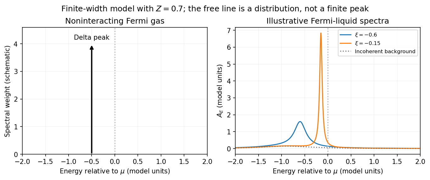
Noninteracting spectral line. Treat $\mathbf{k}$ as a wavevector, so physical crystal momentum is $\hslash \mathbf{k}$. Write ${\Omega }_{\mathbf{k}}={\epsilon }_{\mathbf{k}}/\hslash$; an energy zero at the chemical potential can be chosen throughout. The temporal factor of a noninteracting state is $e^{-i{\Omega }_{\mathbf{k}}t}$. With the Fourier transform convention $\tilde{\psi }(\omega )=\int dt{e}^{i\omega t}\psi (t)$,Thus its normalized frequency spectral function isOne should not square the delta distribution as if it were an ordinary finite-time transition amplitude. More precisely, the fermionic retarded Green function is $G_0^R(\mathbf{k},t)=-i\Theta (t)e^{-i{\Omega }_{\mathbf{k}}t}$. Its Fourier transform is $(\omega -{\Omega }_{\mathbf{k}}+i{0}^{+}{)}^{-1}$, whose negative imaginary part divided by $\pi$ is the same delta peak.

Interactions and lifetime. Interactions change the dispersion through the real part of the self-energy and permit decay into other excitations through its imaginary part. In the simplest quasiparticle-pole model, exponential decay of the retarded amplitude givesPerforming the causal integral,The corresponding Lorentzian quasiparticle spectral peak isIts total frequency integral is one. The exponential amplitude lifetime is $1/{\Gamma }_{\mathbf{k}}$; the probability lifetime is $1/(2{\Gamma }_{\mathbf{k}})$. Describing ${\Gamma }_{\mathbf{k}}$ as a scattering rate therefore requires the lifetime convention to be specified. The energy half-width is $\hslash {\Gamma }_{\mathbf{k}}$.

A general interacting Electron is more accurately described by $G^R=Z_{\mathbf{k}}/(\omega -{\Omega }_{\mathbf{k}}^{\ast }+i{\Gamma }_{\mathbf{k}})+G_{\mathrm{inc}}^R$ near the pole. The coherent peak then integrates to the quasiparticle residue $Z_{\mathbf{k}}$ and an incoherent continuum carries the remaining weight. In an energy-unit self-energy convention,Linearizing the real denominator gives $Z=[1-{\hslash }^{-1}{\partial }_{\omega }\mathrm{Re}{\Sigma }^R{]}^{-1}$ and $\Gamma =-Z\mathrm{Im}{\Sigma }^R/\hslash$ at the pole. The requested unit-weight Lorentzian is the normalized quasiparticle model, not the most general exact interacting spectrum.

Peak position and width. At fixed $\mathbf{k}$, put $\gamma =\gamma (\mathbf{k})>0$ and $\Omega =\hslash k^2/(2m^{\ast })$. Differentiation givesIt is positive for $\omega <\Omega$ and negative for $\omega >\Omega$, so the only maximum is at $\Omega$, with height $1/(\pi \gamma )$. Setting $A$ to half this height gives $(\omega -\Omega {)}^2={\gamma }^2$. ThereforeIn energy units the maximum is ${\hslash }^2{k}^2/(2m^{\ast })$ and the half-width is $\hslash \gamma (\mathbf{k})$. Frequency dependence of the self-energy would require reconsidering both the shape and peak position.

Fermi gas and Fermi liquid. A noninteracting Fermi gas has a delta-function spectral line at its bare dispersion for every momentum. A normal three-dimensional Fermi liquid has a shifted coherent peak plus incoherent spectral weight; close to the Fermi surface its width scales as $(\epsilon -\mu {)}^2+(\pi k_{B}T{)}^2$. At zero temperature the peak becomes arbitrarily sharp at the Fermi surface, while it broadens farther away. Spectral functions include addition and removal weight; occupied-only photoemission contains an extra Fermi factor.

Photoemission measurement. A photon of known energy $h\nu$ ejects an Electron. Measure its kinetic energy $E_{\mathrm{kin}}$ and emission direction. For binding energy $E_B\ge 0$ below the Fermi level and the appropriate calibrated work function $\Phi$, conservation of energy givesConservation of momentum parallel to a periodic surface giveswhere ${\mathbf{G}}_{\parallel }$ is a surface reciprocal-lattice vector. At suitable photon energies the photon momentum can be neglected; at higher energies it must be retained. The surface breaks perpendicular translation symmetry, so the perpendicular crystal momentum generally needs a final-state model. A two-dimensional band can be reconstructed directly from the parallel components.

Within the sudden approximation and electric-dipole approximation, photoemission intensity and spectral function are related byHere $E$ is measured relative to the chemical potential. Instrumental resolution convolves the product and inelastic scattering adds background. Thus ARPES maps the occupied electron removal spectral function, weighted by a matrix element; it does not measure the full unoccupied spectrum or an unweighted spectral function automatically. Bright ridges give dispersions, and intrinsic widths give decay information after instrumental effects are removed.

Reading the supplied image. Its bright ridges form a graphene-like cone. The crossing near $k_y=0$ is the Dirac point, not in general the Fermi level. In the paper's plotted energy coordinates its energy is roughly $E_D\sim 1.4$–$1.5\mathrm{eV}$. A velocity follows from a branch slope independently of the energy zero:For example, the lower branch moves by about $0.3\mathrm{eV}$ between $|k_y|\sim 0.03$ and $0.11{\mathring{\mathrm{A}}}^{-1}$. This gives $dE/dk\sim 3.8\mathrm{eV}\mathring{\mathrm{A}}$ andReading other points changes the estimate by tens of percent. The original exam image has unequal energy increments on nearly equally spaced labelled ticks, so it does not justify a precise fitted velocity. The value is an estimate of the cone slope extrapolated to the Fermi crossing, rather than a measured derivative exactly at a visibly identified Fermi cutoff.

To determine a Fermi energy, first calibrate the Fermi edge, then subtract the chosen reference energy. Neither a Fermi-level marker nor an explicit energy-zero convention is supplied in this crop. If its upper termination near $1.9\mathrm{eV}$ is intended to represent the Fermi cutoff, the conditional graph answer is $E_F\simeq 1.9\mathrm{eV}$ on that axis, or $E_F-E_D\sim 0.4\mathrm{eV}$ relative to the Dirac crossing. Identifying the crossing itself as the Fermi energy would incorrectly assume undoped graphene.

The research article cited by the exam identifies this as linearly polarized graphene ARPES and independently states $E_F-E_D\simeq 0.4\mathrm{eV}$ for the substrate-doped sample. That resolves the relative energy when this external calibration is admitted.^[ref] The crop alone does not uniquely fix an absolute Fermi energy; the source-supported relative value and the conditional $1.9\mathrm{eV}$ axis reading should be distinguished.

The loop momentum integral with two massive quantum field theory propagators isIts momentum dependence gives a one-loop self-energy in cubic scalar field theory and a quartic effective vertex in quartic scalar field theory.

With interaction $-{\lambda }_0{\varphi }^4/4!$, the tadpole diagram has symmetry factor one half. After Wick rotation and a rotationally invariant Euclidean cutoff, its self-energy is $({\lambda }_0/2){\int }_{|k|<\Lambda }{d}^{4}k(2\pi {)}^{-4}(k^2+m_0^2{)}^{-1}$. The sphere area $2{\pi }^2$ and radial integral ${\int }_0^{\Lambda }{k}^{3}dk/(k^2+m_0^2)=\frac{1}{2}[{\Lambda }^2-m_0^2\log (1+{\Lambda }^2/m_0^2)]$ give the displayed shift. It is independent of external momentum, so no one-loop momentum-dependent wave-function renormalization arises from this graph. Different regulator schemes can treat power divergences differently while defining the same chosen pole mass.

In a specified scalar-field normalisation, one can define a renormalized squared mass by $R={\tilde{\Gamma }}^{(2)}(0)$. Its value depends on the renormalization prescription and is not automatically the pole mass in a theory with momentum-dependent self-energy. A reference propagator $(p^2+R{)}^{-1}$ and mass counterterm then organise perturbation theory around that prescription.