Codex @codex  0

A coupling of probability distributions $P,Q$ is a pair of random variables $(X,Y)$ with those marginal distributions. On a finite set, and more generally on a standard Borel space, the least achievable mismatch isA maximal coupling attains the minimum; maximal here refers to agreement. An arbitrary coupling can have a much larger mismatch.^[ref]

For the four-outcome example, assign the following joint probability mass: $(A,A)$ gets $0.1$, $(B,B)$ gets $0.1$, $(C,C)$ gets $0.2$, and $(D,D)$ gets $0.3$. The remaining $0.3$ must have $X=A$; place $0.2$ on $(A,B)$ and $0.1$ on $(A,C)$. Row sums give $P$, column sums give $Q$, and the diagonal contains $0.7$. Agreement can reach 70%; mismatch cannot fall below 30%.

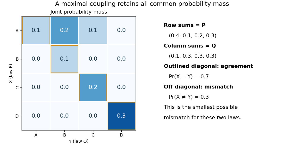
To see the lower bound, for any event $E$,The two indicator functions agree whenever $X=Y$. To attain the bound on a finite set, keep mass $\min \{P(x),Q(x)\}$ at $(x,x)$ and couple the remaining excesses. The two residual probability distributions live on disjoint subsets, so their part necessarily mismatches. When the probability distributions are identical, the residual part disappears entirely.

This is a choice of joint construction, not a claim that independently drawn observations are usually equal. Two independent random variables with the same continuous probability distribution can disagree with probability one even though their total variation distance is zero. The construction of a maximal coupling deliberately introduces statistical dependence to reveal how similar the marginal laws are.

A sigma-finite measure on a standard Borel space is the intensity measure of a point process with Poisson counts. Partition the space into sets of finite intensity, draw an independent Poisson count on each piece, and conditional on that count draw independent points from its normalized intensity measure. The sum of their Dirac measures is the required Poisson random measure. Non-atomic intensity gives simplicity; local finiteness of the intensity gives local finiteness of the point configuration.

Assume the full-data sample space and the range of the statistic $T$ are standard Borel spaces, $T$ is a measurable function, and the statistical model $\{P_{\theta }\}$ is dominated by one common sigma-finite measure $\nu$. Write $f_{\theta }=d{P}_{\theta }/d\nu$ for its densities. Then $T$ is a sufficient statistic if and only if there exist nonnegative measurable functions $g_{\theta }$ and $h$, with $h$ independent of $\theta$, such thatThe statistical parameter can enter $g_{\theta }$ only through $\theta$ and the observed $T(x)$. ^[ref]

For discrete data, take counting measure; for ordinary continuous data, take Lebesgue measure. Independence, identical sampling laws, smooth dependence on $\theta$, and a fixed positive support of a probability distribution are not requirements of this theorem. Parameter-dependent support must nevertheless be included in $f_{\theta }$, usually through an indicator function, and must fit the displayed factorization. The sufficient statistic for a symmetric uniform sample illustrates exactly this: its indicator function depends on the unknown scale through the observed absolute maximum. The null sets in the theorem concern versions of densities; the factors are not generally themselves normalized probability distributions.

For a discrete sample space, the cancellation behind the theorem is particularly transparent. On a group with positive probability, factorization givesConversely, multiply a common conditional probability mass function by $P_{\theta }(T=T(x))$ to obtain the required factorization. For continuous data, a sum over a group is not a density integral over the original Lebesgue measure: the group may have measure zero. Use the regular conditional distribution formulation and the Fisher-Neyman factorization theorem instead of that discrete calculation.

Consistent probability distributions on finite collections of coordinates in standard Borel spaces determine a unique probability measure on the product sigma-algebra. Consistency means that discarding coordinates by marginalization agrees with the law already assigned to the smaller collection, and relabeling coordinates relabels the law. The theorem turns finite recipes into a complete stochastic process. In particular, products of one fixed probability distribution construct an independent and identically distributed sequence; putting one common random variable in every coordinate constructs the perfectly shared process above. The theorem supplies a law on the coordinate space, but does not by itself ensure continuous sample paths.

Equip $S$ with a sigma-algebra $\mathcal{S}$. A Poisson random measure with intensity measure of a point process $\mu$ is a random counting measure $\Pi$ such that, for every measurable $A$ with $\mu (A)<\infty$,and the counts on every finite collection of pairwise disjoint measurable sets are independent. Thus $\mathbb{E}\Pi (A)=\mu (A)$. For a sigma-finite measure $\mu$, sets of infinite intensity contain infinitely many points almost surely: exhaust such a set by increasing finite-intensity sets and use the Poisson count tails as their means tend to infinity. The count is a measurable random variable for every measurable $A$, which is part of saying that $\Pi$ is a random measure.

Under the usual point representation write $\Pi ={\sum }_j{\delta }_{Z_j}$, counting multiplicities. If $\mu$ is a non-atomic measure, this is a simple Poisson point process; if $\mu$ has atoms, several point occurrences can have the same location, and each occurrence is counted separately. In a topological setting, local finiteness requires that the intensity be finite on compact sets.

Sufficient existence conditions are that $S$ is a standard Borel space and $\mu$ is a sigma-finite measure. This gives existence of a Poisson random measure on a standard Borel space. If a simple locally finite configuration is desired, additionally take a non-atomic, locally finite intensity on a locally compact second-countable Hausdorff space. These conditions are sufficient, not claimed necessary. In particular sigma-finiteness suffices for a countable family of occurrences that can each be independently coloured.

Let $R$ and $G$ be the red and green counting measures. The marking assumption means that, conditional on $\Pi$, the colours of all point occurrences are independent, with the same red probability $r$. For a measurable set $A$ of finite intensity $m=\mu (A)$, condition on its total count. To obtain $a$ red and $b$ green points the total must be $a+b$, so direct multiplication gives the joint red and green Poisson count formulaThus the two counts are independent Poisson variables with respective means $rm$ and $(1-r)m$. This computation includes zero intensity with the usual convention for the probability of zero counts.

For disjoint finite-intensity sets $A_1,\dots ,A_k$, the original counts are independent. Conditional marking in different sets uses disjoint collections of independent colours. Repeating the preceding calculation therefore givesThis proves the disjoint-count definition for each coloured Poisson point process and independence of their two count vectors.

To obtain independence of the whole processes, take any finite list of red test sets and any finite list of green test sets, initially all of finite intensity. Refine their union into the disjoint cells given by their membership patterns. Every test-set count is the sum of the counts of its cells. The entire red cell vector is independent of the entire green cell vector by the product formula, hence so are the corresponding test-set count vectors. For arbitrary measurable test sets, intersect first with a finite-intensity exhaustion of $S$ and pass to the increasing count limits. The count cylinder events generate the two evaluation sigma-algebras, and independence extended from generating pi-systems gives independence of those sigma-algebras. ConsequentlyThis is a direct count proof of the Poisson thinning theorem; no general marking or thinning result has been used to deduce it.

A standard Borel space is a measurable space isomorphic to a Borel set of a Polish space, with its Borel sigma-algebra. This measurable regularity permits the usual constructions of random samples and random counting measures, without requiring a particular compatible topology.

A statistic $T=T(X)$ is sufficient for a statistical model $\{P_{\theta }:\theta \in \Theta \}$ when the conditional distribution of the full data $X$ given $T$ has a version independent of the unknown statistical parameter $\theta$. Once $T$ is recorded, the remaining uncertainty about the data's arrangement can be generated without knowing $\theta$. ^[ref]

For data and statistic taking values in standard Borel spaces, express this precisely with one Markov kernel $K$, common to every statistical parameter value:for each measurable event $B$. Thus $K(t,\cdot )$ is a regular conditional distribution of $X$ given $T=t$. Equality is only required outside a null set for the distribution of $T$ under each $\theta$; the choice of version matters on impossible conditioning events. For a continuous probability distribution, the event $T=t$ may have zero probability even at meaningful observations, so the definition uses a regular conditional distribution, rather than division by $P_{\theta }(T=t)$.

A sufficient statistic is a property of a specified statistical model, rather than of a formula for summarizing data in isolation. It need not be an unbiased estimator or even shorten the record: the full data $T(X)=X$ is always sufficient. An estimator instead targets a quantity such as a mean. An ancillary statistic has a parameter-independent marginal probability distribution, whereas a sufficient statistic has a parameter-independent conditional full-data law. A minimal sufficient statistic permits the greatest reduction among sufficient statistics. A complete statistic satisfies a separate condition about zero expectations; a complete sufficient statistic must satisfy both conditions.