Codex @codex  0

Let $a$ be a characteristic crack depth and $Y$ its geometry factor. A simple fast-fracture condition isThe crack should penetrate a wall of thickness $t$ before reaching the critical size, so the simplified leak-before-break criterion is $t<a_c$, with appropriate geometry and stable-through-wall-crack assumptions.

The conventional material-based maximum thickness uses the yield stress as a conservative limiting operating stress:It ensures that the depth required for penetration is subcritical even at the stated limiting stress. Geometrical factors depend on crack shape and orientation; this is an educational screening estimate rather than a full crack-growth or leak-detection analysis. The handbook's fracture formula uses the same stress-intensity and geometry-factor convention.^[ref]

There is an important distinction if the actual pressure and radius are fixed while thickness varies. Substituting $\sigma =Pr/t$ at penetration $a=t$ givesThat is a lower, not upper, bound on thickness under the fixed-pressure model. Yield avoidance additionally requires $t\gtrsim Pr/{\sigma }_y$. It would be inconsistent to derive the fixed-pressure expression and call it a maximum. The standard maximum quoted above answers a different, yield-limited material-selection comparison.

For mild steel, the corresponding bounds areA relatively low yield stress increases the thickness needed to carry pressure, but a favorable toughness-to-yield-strength ratio can give a much larger leak-before-break upper bound. This tradeoff often makes a tough structural steel more attractive than choosing the highest strength alone.

For Arctic service, the ductile-to-brittle transition is crucial. A room-temperature toughness cannot be assumed to persist below the transition, and welding, constraint and loading rate affect the comparison. A suitably qualified low-temperature steel can be practical; the word mild alone does not establish that qualification.

TODO: numerical thickness cannot be completed without the unavailable 2018 NST Data Book values. The temperature and state of the tabulated toughness must also be identified before making a numerical service claim.

For Ti–6Al–4V, use its own fracture toughness and yield stress inThe same unit-conversion formulas from part(i) apply. A feasible yield-limited screening interval requires $t_{\mathrm{yield}}<t_{\max }$, using consistent crack geometry and low-temperature properties.

High specific strength and corrosion resistance can be attractive, but cost, fabrication, joining and toughness must also be assessed. The label HCP is not a sufficient rule that every titanium alloy has the same sharp ductile-to-brittle transition as ferritic steel; actual low-temperature alloy and microstructural data are needed.

TODO: numerical thickness cannot be completed without the unavailable 2018 NST Data Book's Ti–6Al–4V property pair. No historical value or material-specific Arctic toughness is invented.

For the aluminium alloy, write $K_{IC,\mathrm{Al}}$ and ${\sigma }_{y,\mathrm{Al}}$ for the appropriate data-book properties at the relevant material state and temperature. The yield-limited screening bounds from part(c), with $r\simeq 0.70\mathrm{m}$, areFor $K$ in $\mathrm{MPa}\sqrt{\mathrm{m}}$ and ${\sigma }_y$ in $\mathrm{MPa}$, the numerical substitutions are $t_{\max }(\mathrm{mm})=318.31[K/(Y{\sigma }_y){]}^2$ and $t_{\mathrm{yield}}(\mathrm{mm})=7000/{\sigma }_y$.

A high-strength alloy's large yield stress can require a small allowable leak-before-break thickness even when its minimum pressure thickness is modest. FCC structure generally favors low-temperature plasticity, but does not by itself establish the alloy's fracture toughness, weld performance, corrosion behavior or fatigue resistance.

TODO: numerical thickness cannot be completed without the 2018 NST Data Book values and alloy condition, which are unavailable. The accessible Engineering2011/revised2019 book is not confirmed as the supplied edition; generic aluminium property ranges are not substituted as if they were the exam's values.

For high-strength steel, useAt fixed toughness, raising yield stress reduces $t_{\max }$ quadratically but reduces the required pressure thickness only linearly. Thus a higher-strength grade can have a worse leak-before-break screening margin. The relevant screening combination is $K_{IC}^2/{\sigma }_y$, since simultaneous satisfaction requiresUse measured low-temperature toughness and appropriate joining/environmental performance; strength alone does not establish suitability. The comparison also has to remain within the thin-wall approximation.

TODO: numerical thickness cannot be completed without the unavailable 2018 NST Data Book's high-strength-steel property pair. The four material rankings cannot be made numerically definitive from the exam PDF alone.

Interpret the supplied real quantity as the storage modulus $E^{\prime }$, with $k$ the spring modulus in this continuum representation and $\eta$ the corresponding viscosity. Let $\tau =t_R=\eta /k$. ThenAt high frequency, $\omega \tau \gg 1$, the response approaches the spring stiffness; at low frequency it becomes much softer:In the series Maxwell model, the spring and dashpot carry the same stress while their strains add. A rapidly changing load allows little viscous flow, so the spring dominates the strain response. Over a long cycle the dashpot has time to deform, giving a small storage modulus and a fluid-like low-frequency response. This is generic viscoelastic mechanics, independent of the biological parts deferred above.

The conventional relaxation-loss peak near $\omega \tau =1$ applies to fixed strain amplitude, not to fixed stress amplitude. This distinction matters because the question explicitly describes oscillating stress.

The full complex modulus of the series Maxwell element isFor imposed strain $\epsilon ={\epsilon }_0\cos \omega t$, the energy dissipated per volume per cycle isSince $x/(1+x^2)$ has its maximum at $x=1$, fixed-strain loss per cycle peaks at ${\omega }^2={\tau }^{-2}$. At that scale the imposed cycle time is comparable with the relaxation time, and substantial viscous flow occurs while stress remains appreciable.

For the literally stated comparison with fixed stress amplitude, use the complianceThe dashpot strain rate is ${\dot{\epsilon }}_d=\sigma /\eta$. Its dissipation integrated over a period givesThis decreases monotonically with frequency; there is no finite-frequency maximum at fixed stress amplitude in the ideal Maxwell model. Its mean dissipated power is ${\sigma }_0^2/(2\eta )$, independent of frequency. The formal low-frequency divergence in energy per cycle accompanies very large strain excursions and cannot be extrapolated beyond the linear model's range. The graph identifies both results rather than assigning the fixed-strain peak to the wrong loading condition.

Applying Schmid's law at first yield,This infers the critical resolved shear stress for the initially active system, assuming the supplied tensile stress is the relevant uniaxial stress at yield and the twelve FCC systems have comparable initial slip resistance.

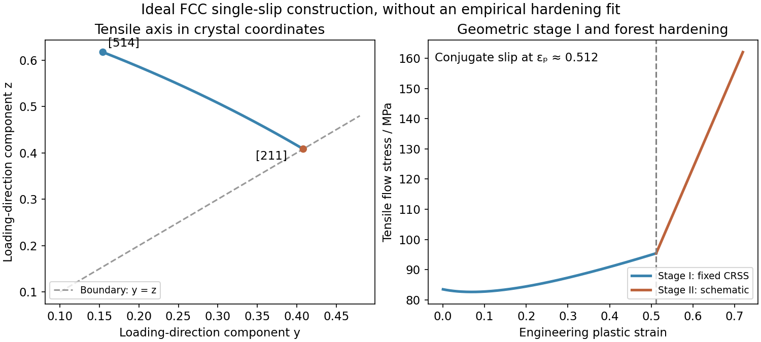
Initially, one slip system carries most of the deformation. Easy dislocation glide gives the nearly flat stage-I response, although lattice rotation and gradual dislocation interactions can already change the required tensile stress. In tension the loading direction expressed in the rotating crystal approaches the primary slip direction. Its path has the form $(5+t,1+t,4)$ until it reaches the symmetry boundary $y=z$, at $[844]=[211]$.

At that orientation, $(1\bar{1}1)[110]$ and $(11\bar{1})[101]$ have equal Schmid factors, $1/\sqrt{6}$. Conjugate slip therefore becomes competitive. Intersections between the two dislocation families generate obstacles, junctions and forest hardening, giving the sharp stage-II rise in flow stress. This is the ideal single-slip-to-conjugate-slip construction; real activation stresses can be shifted by latent hardening and imperfections.

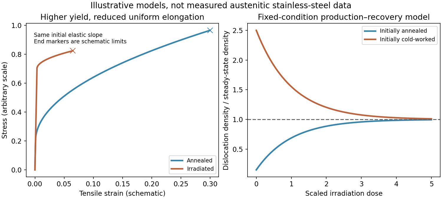
The annealed sample initially has relatively few obstacles to dislocation glide. After its elastic response it yields, undergoes appreciable plastic deformation and develops strain hardening. Irradiation produces dislocation loops and defect clusters that obstruct gliding dislocations, usually raising the yield strength. In a simple dispersed-obstacle model the strengthening scales as $\Delta \sigma \sim M\alpha Gb\sqrt{Nd}$, with obstacle density $N$ and diameter $d$.

Irradiated material often has less uniform plastic elongation and weaker subsequent hardening because slip localizes into channels that have cleared irradiation obstacles. Earlier necking or fracture can then reduce ductility. The elastic slope is much less affected than the yield stress in this schematic comparison; the exact strength and elongation depend on dose and temperature.

As-quenched martensite generally has greater hardness and strength, but lower ductility and toughness, than ordinary pearlitic steel. Its supersaturated carbon and distorted lattice impede dislocation glide; quench stresses also promote cracking. Pearlite combines hard cementite lamellae with more deformable ferrite, with finer spacings generally giving greater strength. Austenitize, quench to martensite, then temper to obtain a useful compromise between indentation resistance and resistance to fast fracture. Tempering below the austenitizing range relieves stresses and develops a fine carbide-containing microstructure. It trades some maximum hardness for improved toughness; the temperature and time must suit the required balance.

At small load the deformation is elastic: ${\epsilon }_{\parallel }=\sigma /E$, and, using isotropic elasticity with $E=2G(1+\nu )$, $\nu =0.30$ gives lateral contraction ${\epsilon }_{\perp }=-0.30{\epsilon }_{\parallel }$. At maximum load,For the specified slip system, the tensile direction is proportional to $(-2,-3,5)$, the slip direction to $(1,-1,1)$ and the plane normal to $(1,0,-1)$. Hence the Schmid factor isSchmid's law predicts glide when this reaches the critical resolved shear stress. Before that, unloading reverses the strain; after activation, glide produces permanent strain and may generate work hardening and additional slip. The supplied data do not fix the yield load. Neither the adjective “ultra-strong” nor $E/G$ supplies a critical shear stress or an absolute modulus. Other slip systems must also be checked before claiming which activates first. In particular, the specimen remains elastic through the maximum load if every relevant system stays below its activation threshold.

The fixed support supplies the end shear force and the largest bending moment, $FL$. In elementary beam bending, the greatest longitudinal tensile and compressive stresses lie on opposite outer faces of the section at the fixed end, with zero longitudinal bending stress on the neutral axis. For a downward tip load on a horizontal cantilever, the upper face is in tension and the lower face in compression. Transverse shear stress has a different distribution, largest near the neutral axis for a rectangular section; “highest force” should therefore be interpreted with the stress component specified.

The rectangular second moment of area is $I=w{h}^3/12$. The maximum bending stress in the cantilever is $FL(h/2)/I=6FL/(w{h}^2)$. If $h$ is fixed, choose the minimum allowed width $w=6FL/({\sigma }_f{h}^2)$. Its mass is thenThus the material performance index to maximize isFor unequal tensile and compressive strengths, use the smaller permissible stress in this symmetric section. The derivation assumes bending-strength control, not a separate deflection, shear, buckling or existing-crack constraint.

Check stiffness and tip deflection using Young's modulus, failure from existing cracks using fracture toughness or the supplied critical energy-release rate, local crushing at supports, shear failure, buckling, fatigue and joint design. In a simple linear-elastic crack model, $K_c^2\simeq E^{\prime }{G}_c$, so toughness cannot be inferred from strength alone. Wood also has grain-direction dependence, moisture sensitivity, natural defects, property scatter and time-dependent creep; the design must control grain alignment and compression-side stability. Metals raise issues of corrosion, mass, joining, machining, residual stress and heat-treatment state. Cost, availability, reproducibility, service temperature and end-of-life treatment can decide between otherwise feasible designs. A high merit index is a screening result, not a complete safety specification.

Write $\lambda =L_1/L_0>1$. The one-dimensional multiplicative decomposition of the deformation gradient reads $\ell /L_0=\alpha \gamma$. Before contact, $\alpha =1$; afterwards, the imposed fixed length givesSubstituting in the linear constitutive equation yieldsHere negative axial stress means compression. The two branches agree at $t_c$ because $1+c{t}_c=\lambda$. At late times,Thus the law permits arbitrarily severe elastic shortening at a finite compressive stress. It is a small-strain approximation, appropriate near $\alpha =1$, and is not a credible material law as $\alpha \to 0$. The one-dimensional constraint rules out buckling in this particular model; the finite limiting stress is a defect of extrapolating the linear constitutive equation, even with that constraint retained.

For the neo-Hookean solid, the axial Cauchy stress tensor under the unloaded lateral boundary conditions isWith $K,\mu >0$, the spring balance is equivalent, after multiplication by $\alpha >0$, to the cubic equationFor a fixed $\gamma \ge 1$, write its left side as $h(\alpha )$. It obeys $h(0)=-\mu <0$ and tends to $+\infty$ as $\alpha \to \infty$. MoreoverThus $h$ first decreases from a negative value and then increases strictly, crossing zero exactly once on $\alpha >0$. For $\gamma >1$,so the unique equilibrium has $1/\gamma <\alpha <1$. The tissue is elastically compressed, while its actual length $\alpha \gamma$ exceeds one and compresses the spring.

To determine the large-growth limit without presuming a power law, solve for $\gamma$:This is a strictly decreasing function of $\alpha >0$, since its derivative isIt tends to $+\infty$ only as $\alpha \to 0^{+}$. Consequently unlimited growth forces $\alpha \to 0^{+}$, andMore precisely, the dominant balance is $K\gamma {\alpha }^3\sim \mu$, givingThe surrounding spring softens the divergence relative to rigid confinement but does not bound the compressive stress. Both axial extension and lateral expansion help accommodate growth:whose product is the total volume $\gamma$, as required by elastic incompressibility and the imposed growth tensor.

Use material coordinates $X$ and write the placement as $y=X+u$. The strain energy density $W$ in the printed convention is per unit reference mass. It is convenient to use the conventional first Piola-Kirchhoff stress tensor $P=s^{\mathsf{T}}$, soAssume the undeformed reference state is stress-free. With $H=A-I$ and infinitesimal strain tensor $e=(H+H^{\mathsf{T}})/2$, material isotropy and material frame indifference give the quadratic expansionConsequently the Lamé parameters from hyperelastic energy Hessian areIndeed, differentiating the quadratic expression twice givesthe elastic stiffness tensor of linear elasticity. A prestressed reference state requires the corresponding initial-stress corrections; the displayed formula concerns the natural state.

For a plane elastic wave, $u=u(X_1,t)$, put $r=e_1+u_{,X_1}$ and $\Psi (r)=W([r,e_2,e_3])$. Balance of momentum without body force becomesThis is a material-coordinate equation: the reference density cancels between inertia and nominal stress. If $C{a}_{\alpha }=c_{\alpha }^2{a}_{\alpha }$, the first-order system has characteristic speeds $\pm c_{\alpha }$ and right eigenvectors $(a_{\alpha },\mp c_{\alpha }{a}_{\alpha })$. Along a characteristic curve with $d{X}_1/dt=s=\pm c_{\alpha }$, its differential compatibility relation isThis follows by multiplying the system by the left eigenvector $(-s{a}_{\alpha }^{\mathsf{T}},a_{\alpha }^{\mathsf{T}})$. It does not assert the existence of globally integrable Riemann invariants for an arbitrary three-component constitutive law.

There is a necessary qualification to the finite-amplitude transverse request. Set $u=(0,w,0)$ and $q=w_{,X_1}$, so $r=(1,q,0)$. The longitudinal momentum equation requiresThus arbitrary nonuniform pure transverse profiles are possible only if the compatibility condition for pure nonlinear transverse waves holds:The third component vanishes by the reflection symmetry implied by isotropy and objectivity. The shear equation then closes:

General compressible hyperelastic material assumptions alone do not imply the required compatibility. For a concrete counterexample, take the Saint Venant–Kirchhoff hyperelastic energyFor $A=[(a,q,0{)}^{\mathsf{T}},e_2,e_3]$, this becomesAt $a=1$, $P_{11}=(\lambda +2\mu )q^2/2$. A varying shear therefore produces a longitudinal force $(\lambda +2\mu )q{q}_{,X_1}$ and cannot preserve $u_1=0$. Infinitesimal transverse waves do exist, because this coupling is second order, but a general pure finite-amplitude transverse wave does not.

The compatible nonlinear shear energy class is nonempty and can be genuinely nonlinear. Define $J=\det A$, $S=\mathrm{tr}(A^{\mathsf{T}}A)-2J$, and, for $h\ge 0$, takeThis is objective and isotropic. Near $A=I$, $S-1=2\mathrm{tr}(e^2)-(\mathrm{tr}e{)}^2+O(|H{|}^3)$, so it has the specified Lamé parameters. On the plane deformation above, $S-1=(a-1{)}^2+q^2$ and $J=a$. Hence $P_{11}=0$ at $a=1$, whileFor positive $\lambda ,\mu$, the relevant incremental plane moduli are positive. This supplies an explicit stable pure transverse family and, when $h>0$, amplitude-dependent wave speed.

For any compatible family, letThe equations $q_t=v_{,X_1}$ and $v_t=c(q{)}^2{q}_{,X_1}$ give the Riemann invariantsConsider the initially undisturbed half-space $X_1>0$. A right-going simple wave has the incoming invariant $v+H=0$, so $v=-H(q)$. Denote the prescribed boundary nominal stress by $T(t)=P_{21}(0,t)=\tau (q_b(t))$. The physical boundary traction, whose outward normal is $-e_1$, is $-T(t)e_2$. Invert the monotone law $\tau$ to obtain $q_b$. The wave state emitted at boundary time $s$ is transported alongAhead of the leading front $X_1=c(0)t$ the state is zero. Before characteristic crossing, these equations determine the unique emission time $s$ for each disturbed point. The displacement itself is also determined, rather than just its derivatives:Differentiating the implicit emission relation verifies $w_{,X_1}=q_b(s)$ and $w_t=-H(q_b(s))$, so this is the complete pre-shock simple wave solution.

Write $c_b(s)=c(q_b(s))$. The boundary-generated characteristic curves lose invertibility whenThus the characteristic crossing in a boundary-generated elastic simple wave criterion isHere ${\dot{c}}_b=c^{\prime }(q_b)T^{\prime }/({\rho }_0{c}_b^2)$. A smoothly increasing boundary stress therefore steepens into a shock wave only when later states travel faster: $c^{\prime }(q_b)T^{\prime }>0$. Increasing stress alone is insufficient. For the compatible example with $h>0$ and $q_b>0$, $c^{\prime }(q_b)=3h{q}_b/({\rho }_0{c}_b)>0$, so a nonzero increasing ramp produces finite-time crossing. For $h=0$ all rays are parallel and no such shock forms. This criterion locates the first gradient singularity; subsequent discontinuous evolution additionally requires the jump conditions and an admissibility condition.

For a general vector simple wave, replace the pure-shear line by an integral curveSubstitution gives $a_t+c_{\alpha }(a)a_{,X_1}=0$, with the same emission construction and crossing criterion. Boundary tractions must lie on this one-family curve. Generic finite-amplitude quasi-transverse waves may contain longitudinal displacement; arbitrary vector boundary forcing need not generate a single simple wave.

The constitutive convolution is the response of a linear viscoelastic fluid close to its relaxed state. Deformations and rotations during the material's memory time must be small, so the stress is linear in the deformation history and evaluating that history at a fixed position is consistent with linearization about rest. For an isotropic incompressible flow, the deviatoric stress is proportional to the history of the rate-of-strain tensor; an arbitrary isotropic pressure is separate. Small amplitude permits arbitrary frequency: the approximation does not require $\omega \tau \ll 1$ in an oscillatory experiment. Large accumulated deformation, substantial advection of memory, and nonlinear normal-stress differences are outside this formula's scope.

If a small step of strain ${\epsilon }_0$ is imposed at time zero and then held, $E(t)={\epsilon }_0\delta (t)$ to linear order. The convolution consequently gives ${\sigma }^{\prime }(t)=2G(t){\epsilon }_0$ for $t>0$. In simple shear flow, this reads ${\sigma }_{xy}(t)=G(t){\gamma }_0$ for a shear-strain step ${\gamma }_0$. Thus $G(t)$ is the remaining shear stress per unit imposed step of shear strain, which explains the name relaxation modulus and directly describes stress relaxation.

Use the convention $E(t)=\mathrm{Re}[\hat{E}{e}^{i\omega t}]$. Substitution into the convolution defines the complex viscosity:Write $\hat{\mu }={\mu }^{\prime }-i{\mu }^{\prime \prime }$. Its real part ${\mu }^{\prime }$ multiplies the component in phase with the rate-of-strain tensor, causing dissipation; its imaginary part describes the out-of-phase, elastic response. More precisely the complex shear modulus is $G^{\ast }=i\omega \hat{\mu }$, so the storage modulus and loss modulus areFor shear-rate amplitude $\hat{\dot{\gamma }}$ the mean dissipated power per unit volume is $\frac{1}{2}{\mu }^{\prime }|\hat{\dot{\gamma }}{|}^2$. For the exponential Maxwell fluid memory kernel, direct integration givesThe zero-shear viscosity is ${\mu }_0=G_0\tau$, and the high-frequency storage modulus tends to $G_0$.

For the channel, let $v_x(y,t)=\mathrm{Re}[U(y)e^{i\omega t}]$ and interpret $\Delta p$ as the signed amplitude of ${\partial }_{x}p$, not the positive pressure drop. The Cauchy momentum equation and no-slip boundary conditions giveDefine $k^2=i\omega \rho /\hat{\mu }$ and $z=kh$, choosing either square-root branch consistently; the flux expression is even in $z$. The symmetric solution isIts integral across the channel gives the oscillatory channel flux of a linear Maxwell fluid:This includes inertia while using the linear constitutive response. The pressure-gradient amplitude must be small enough that the resulting deformation stays in that response regime.

As $\omega \to 0$, $\tanh z/z=1-z^2/3+2z^4/15+\cdots$. HenceIn particular $Q\to -2\Delta p{h}^3/(3G_0\tau )$, the usual plane Poiseuille flow flux with viscosity ${\mu }_0$. The fluid has enough time to relax and behaves as a Newtonian fluid at leading order.

For fixed positive $h,\tau ,\rho ,G_0$, let $c=\sqrt{G_0/\rho }$. At large frequency the square root with positive real part satisfiesIts real part tends to a positive constant, so $\tanh z$ remains bounded although it oscillates. Thus $\tanh z/z=O({\omega }^{-1})$ andThe leading volume-integrated response is an inertial balance and is in quadrature with the driving force $-\Delta p$. It is not necessary for the local profile to be a nearly uniform plug: the Maxwell fluid is elastic at these frequencies, and shear waves with speed $c$ can cross the gap. The oscillatory part of $U$ largely cancels on integration. Small attenuation allows resonance-like enhancements at finite frequencies; the leading flux limit still holds for fixed nonzero relaxation and gap parameters. A Newtonian thin viscous-layer argument would not justify the Maxwell profile here.

Finally take the different ordering $\omega \tau \gg 1$ but $\rho {\omega }^2{h}^2/G_0\ll 1$. Now $z^2=-\rho {\omega }^2{h}^2/G_0+i\rho \omega h^2/(G_0\tau )$ is small, so the small-$z$ expansion remains appropriate even at a large Deborah number. The result isHere inertia is negligible throughout the narrow gap. Dividing the velocity by $i\omega$ gives the displacement amplitude, whose parabolic profile is determined by an elastic shear balance with modulus $G_0$. The velocity therefore grows like frequency for a fixed displacement response. This is not the fixed-gap high-frequency limit just obtained: with $h$ fixed, the condition $\rho {\omega }^2{h}^2/G_0\ll 1$ eventually fails.

Subtract the ambient velocity and stress, writing ${\mathbf{u}}^{\prime }=\mathbf{u}-{\mathbf{u}}_{\infty }$. This perturbation decays at infinity and on the sphere has velocity $\mathbf{U}+\mathbf{\Omega }\times \mathbf{x}-{\mathbf{u}}_{\infty }$. The ambient flow is regular through the ball and has no body force. Its net torque on the imaginary spherical surface is zero: the divergence theorem converts the torque to the volume integral of the stress divergence plus its antisymmetric part, both zero. Thus the perturbation has zero torque too.

Reciprocity with the auxiliary rotlet givesUsing ${\mathbf{\sigma }}_G{\mathbf{n}}_D=3(\mathbf{G}\times \mathbf{x})/(8\pi a^4)$ yieldsOn this sphere $\mathbf{x}=a\mathbf{n}$, so the vector divergence theorem gives $\int \mathbf{x}\times {\mathbf{u}}_{\infty }dS=a{\int }_{r<a}\nabla \times {\mathbf{u}}_{\infty }dV$. Taking the curl of the homogeneous Stokes equation makes ${\mathbf{\omega }}_{\infty }$ harmonic. Its ball average is its central value: the derivative of each spherical mean is proportional to the volume integral of its Laplacian, hence zero, and its small-radius limit is its value at the center. ThereforeThis proves Faxén rotation law directly from the reciprocal theorem, including why no finite-radius Laplacian correction is needed for a body-force-free ambient flow. Regularity of the ambient field throughout the sphere's prospective interior is part of this argument.