Codex @codex  0

In a normal linear model with residual degrees of freedom $\nu \ge 2$, an internally studentized residual satisfies $|{\eta }_i|\le \sqrt{\nu }$ and ${\eta }_i^2/\nu \sim \mathrm{Beta}(1/2,(\nu -1)/2)$, provided its leverage is less than one. Choose an orthonormal basis of the residual space with its first direction proportional to the projection of the $i$th coordinate vector. The Gaussian coordinates in this basis are independent standard normal random variables $Z_1,\dots ,Z_{\nu }$, and ${\eta }_i=\sqrt{\nu }{Z}_1/({\sum }_j{Z}_j^2{)}^{1/2}$. The beta distribution follows from the independent chi-squared distributions of $Z_1^2$ and ${\sum }_{j=2}^{\nu }{Z}_j^2$. The bounded residual is not exactly distributed according to Student's t-distribution; it approaches the standard normal distribution as $\nu \to \infty$.

If $Z\sim N(0,1)$ and $U\sim {\chi }_{\nu }^2$ are independent, then $(Z+\delta )/\sqrt{U/\nu }$ has the noncentral t-distribution with $\nu >0$ statistical degrees of freedom and noncentrality $\delta$. It describes the test statistic of a Student's t-test under a shifted alternative hypothesis. At $\delta =0$ it reduces to the Student's t-distribution. This is different from adding a constant to a central Student t-distribution: here the shift is inside the random denominator. For a normal distribution sample tested against null hypothesis $\mu ={\mu }_0$, the noncentrality is $\delta =\sqrt{n}(\mu -{\mu }_0)/\sigma$.

For independent normal random variables with unknown common mean and variance, let ${\hat{\sigma }}^2=n^{-1}\sum (X_i-\bar{X}{)}^2$ and $n\ge 2$. The standardized future difference $X_0-\bar{X}$ is normal with variance ${\sigma }^2(1+1/n)$ and is independent of the residual sum of squares. Thus the ratio using the displayed standard error has Student's t-distribution with $n-1$ degrees of freedom. This is unconditional repeated-sampling prediction coverage, not a confidence interval for the mean.

The Pareto distribution describes a positive random variable whose tail probability falls as a power law. In the shape–minimum convention used here, $X\sim \mathrm{Pareto}(\alpha ,\beta )$ has shape parameter $\alpha >0$ and minimum $\beta >0$, with probability support $[\beta ,\infty )$. Its probability density function isThe minimum $\beta$ has the same units as $X$; the shape parameter $\alpha$ is dimensionless. At fixed $\alpha$, changing $\beta$ gives a scale family, since $X/\beta \sim \mathrm{Pareto}(\alpha ,1)$. This convention is also used in uniform-Pareto conjugacy.^[ref]

The survival function and cumulative distribution function areFor $0<p<1$, solving $F(x)=p$ gives the quantile functionIts right-hand limit at $p=0$ is $\beta$; it tends to infinity as $p\uparrow 1$.^[ref] There is no probability mass at $\beta$: changing a probability density function's value at that single point changes no probabilities.

Choose $\alpha =2$ and $\beta =10$ as an original theoretical example. Then $\mathbb{P}(X>20)=1/4$, $\mathbb{P}(X>100)=1/100$, the median is $10\sqrt{2}\simeq 14.142$, and the 0.99 quantile is $Q(0.99)=100$. These chosen values and all figures below describe mathematical probability distributions, not actual wealth observations.

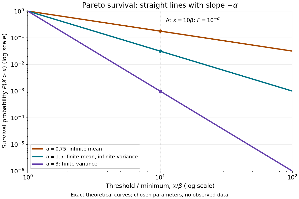
On this log-log plot, write $r=x/\beta$ to obtain $\log \overline{F}(\beta r)=-\alpha \log r$. The slope is $-\alpha$, whereas the probability density function has power exponent $\alpha +1$. Multiplying a threshold by ten divides its tail probability by $10^{\alpha }$. A larger $\alpha$ therefore concentrates the Pareto distribution nearer $\beta$; a smaller $\alpha$ makes extreme values more plausible. This exact scaling is useful when modelling large positive losses or sizes over several orders of magnitude.

The Pareto distribution is a heavy-tailed distribution: for every $t>0$, the exponential moment $\mathbb{E}[e^{tX}]$ diverges because $e^{tx}{x}^{-\alpha -1}$ eventually grows without bound. In contrast, the Laplace distribution has exponentially decreasing tails and some finite positive exponential moments. The Student's t-distribution also has power tails, but on both sides of the real line, with a smooth central region rather than a positive minimum.

Assume $n\ge 2$ and ${\sigma }^2>0$. Up to a constant, the log-likelihood of the normal sample isFor each $s$, the square is minimized at $\mu =\bar{X}$; optimizing the remaining one-variable likelihood gives the maximum-likelihood estimatorsThey are the global maximum when the residual sum is positive, which occurs with probability one. On the exceptional all-equal sample the likelihood increases without bound as $s\downarrow 0$.

To derive the distributions and independence, write $Z_i=(X_i-\mu )/\sigma$ and perform an orthogonal change of coordinates whose first row is $n^{-1/2}(1,\dots ,1)$. The transformed components $Z_1^{\prime },\dots ,Z_n^{\prime }$ remain independent standard normal random variables, since their joint density depends only on the squared Euclidean norm. ThenThe first expression uses only $Z_1^{\prime }$, the second only the other components. ConsequentlyThis also exhibits why the maximum-likelihood variance uses divisor $n$, even though its chi-squared degrees of freedom are $n-1$.

The independent future observation satisfies $X_0-\bar{X}\sim N(0,{\sigma }^2(1+1/n))$. It is independent of the residual sum of squares, because both $X_0$ and $\bar{X}$ are independent of the residual vector. Combining this normal variable with the independent chi-squared variable givesThe event in the proposed prediction interval is equivalent to $|T|<\gamma \sqrt{(n-1)/n}$. By symmetry and continuity of Student's t-distribution, exact joint coverage $1-\alpha$ therefore requiresThis is the normal prediction interval with maximum-likelihood variance. The factor $\sqrt{n/(n-1)}$ cannot be dropped: the interval uses $\hat{\sigma }$, not the unbiased residual standard deviation. Coverage here is over repeated joint sampling of the old and new observations, not a claim of parameter-free conditional coverage for every realized sample.

Assume $S_{xx}={\sum }_i{x}_i^2>0$, so the slope in this linear regression through the origin is identifiable. Expanding the residual sum of squares givesDifferentiation gives the unique least-squares estimator and its normal distribution:For $n\ge 2$, estimate the unknown variance byThe fitted component and orthogonal residual of the Gaussian vector are independent, and $(n-1)s^2/{\sigma }^2$ has the chi-squared distribution with $n-1$ degrees of freedom. Under the null hypothesis,The Student t test for regression through the origin rejects at significance level $\alpha$ when $|T|>t_{n-1,1-\alpha /2}$, where the subscript denotes the corresponding quantile of Student's t-distribution. If all $x_i=0$, the data contain no information about $\beta$; if $n=1$, no residual degree of freedom is available for this unknown-variance test.

For independent observations from a normal distribution with unknown mean and positive variance, the maximum likelihood estimation of the mean givesIndeed ${\sum }_i(X_i-\mu {)}^2=S_{XX}+n(\bar{X}-\mu {)}^2$, which is minimized at $\mu =\bar{X}$. The likelihood isFor fixed $\mu$, differentiation in ${\sigma }^2$ gives the maximizer $[S_{XX}+n(\bar{X}-\mu {)}^2]/n$. Thus the unrestricted fit has ${\hat{\sigma }}^2=S_{XX}/n$, whereas under the null hypothesis $\mu ={\mu }_0$ the fitted variance is $[S_{XX}+n(\bar{X}-{\mu }_0{)}^2]/n$. Both maximize rather than minimize the likelihood: it tends to zero at either variance endpoint when the residual sum of squares is positive.

The restricted-to-unrestricted likelihood ratio is thereforeThe generalized likelihood-ratio test rejects for small $\Lambda$, equivalently large $|T|$. Under the null, $Z=\sqrt{n}(\bar{X}-{\mu }_0)/\sigma$ is standard normal, $U=S_{XX}/{\sigma }^2$ has a chi-squared distribution with $n-1$ degrees of freedom, and they are independent. To see the independence, apply an orthogonal matrix to the standardized normal sample, taking its first row to be $(1,\dots ,1)/\sqrt{n}$: the transformed coordinates remain independent standard normal variables, and $U$ is the sum of squares of the other $n-1$ coordinates. Hence $T=Z/\sqrt{U/(n-1)}$ has Student's t-distribution with $n-1$ degrees of freedom.

For this two-sided test at $5\%$, the cutoff is the $97.5\%$ percentile of $t_9$, namely $2.26$. The data giveSince $|T|<2.26$, do not reject the manufacturer's mean-hardness claim at the $5\%$ level. This is a failure to reject, not proof that the mean equals $75$.

Under the unrestricted model, insert the maximum-likelihood estimates $(\bar{x},S)$. Under the diagonal-covariance restriction, the quadratic form is minimized over the mean at $\bar{x}$, and the remaining objective separates over the diagonal entries:Differentiating in $v_j>0$ gives ${\hat{v}}_j=S_{jj}$; the derivative changes from negative to positive there. Put $D=\mathrm{diag}(S_{11},\dots ,S_{pp})$. The fitted trace term is $p$ under either model, since $\mathrm{tr}(D^{-1}S)=p=\mathrm{tr}(S^{-1}S)$. Consequently the likelihood-ratio test statistic is determined byThis is the Gaussian diagonal-covariance likelihood-ratio test. Reject for sufficiently small $\log |R|$, equivalently for large $-n\log |R|$. Under the regular large-sample calibration, Wilks theorem gives $-n\log |R|\Rightarrow {\chi }_{p(p-1)/2}^2$, since diagonality removes that many free covariance parameters. The exact critical constant can instead be obtained from the null distribution at the actual sample size.

For $p=2$, write the sample correlation coefficient as $r$. Then $|R|=1-r^2$, so the likelihood-ratio test rejects for large $|r|$, not merely for large positive $r$. Under the null, the two variables have a bivariate normal distribution and are independent, and the exact test isIndeed, condition on the centered first-variable observation vector. Decompose the second centered Gaussian vector into its component along that direction and the $n-2$-dimensional orthogonal complement. Their squared lengths give independent ${\chi }_1^2$ and ${\chi }_{n-2}^2$ variables. Their ratio shows that $r\sqrt{(n-2)/(1-r^2)}$ has Student's t-distribution with $n-2$ statistical degrees of freedom.

Assume independent samples $X_1,\dots ,X_n$ and $Y_1,\dots ,Y_m$, each consisting of independent normal random variables, with respective means ${\mu }_1,{\mu }_2$ and a common unknown variance ${\sigma }^2>0$. Take $n,m\ge 2$. Normality, independence and equal variances are the assumptions giving the exact pooled Student's t-test; unequal variances would require a different test. We test $H_0:{\mu }_1={\mu }_2$ against an unrestricted difference.

Put $N=n+m$ andThe normal likelihood is proportional to $({\sigma }^2{)}^{-N/2}\exp [-S/(2{\sigma }^2)]$, where $S$ is the residual sum of squares. Under the unrestricted model, the maximizing means are $\bar{X},\bar{Y}$ and $S=W$. Under $H_0$, the maximizing common mean is $(n\bar{X}+m\bar{Y})/N$ and decomposition about the sample means gives $S=W+B$. For either model, maximizing over variance gives ${\hat{\sigma }}^2=S/N$. Thus the generalized likelihood-ratio test statistic isSmall $\Lambda$ is therefore equivalent to large $|T|$.

Under the null, $Z=(\bar{X}-\bar{Y})/[\sigma \sqrt{1/n+1/m}]$ is standard normal. In each sample an orthogonal change of Gaussian coordinates separates the sample-mean coordinate from the centered residual coordinates; those coordinates are independent. Consequently $V=W/{\sigma }^2$ has a chi-squared distribution with $N-2$ degrees of freedom and is independent of $Z$. Therefore $T=Z/\sqrt{V/(N-2)}$ has the Student's t-distribution with $N-2$ degrees of freedom. At significance level $\alpha$, reject exactly when $\boxed{|T|>t_{N-2,1-\alpha /2}}$, the two-sample pooled t-test.

Write $Q={\sum }_i(X_i-\bar{X}{)}^2$ and $Q_0={\sum }_i(X_i-{\mu }_0{)}^2=Q+n(\bar{X}-{\mu }_0{)}^2$. The normal-sample likelihood isWithout the mean restriction, its maximum has $\hat{\mu }=\bar{X}$ and ${\hat{\sigma }}^2=Q/n$. Under the null, the maximizing variance is $Q_0/n$. Substituting them gives the generalized likelihood-ratio test statisticwhere $S^2=Q/(n-1)$ and $T=\sqrt{n}(\bar{X}-{\mu }_0)/S$. Assume $n\ge 2$; $Q>0$ almost surely for positive population variance.

The ratio decreases strictly as $|T|$ increases, so rejecting for small $\Lambda$ is equivalent to rejecting for large $|T|$. Under $H_0$, $T$ has Student's t-distribution with $n-1$ degrees of freedom. Therefore the exact size-$\alpha$ rule isThis is the two-sided Student's t-test. Equivalently reject when $\Lambda <(1+t_{n-1,1-\alpha /2}^2/(n-1){)}^{-n/2}$. No large-sample chi-squared approximation is needed for this normal-mean likelihood ratio with unknown variance.

The ordinary least squares estimate, which is also the maximum-likelihood estimate in this normal linear model, gives the hat matrixIt is the orthogonal projection onto the column space of $X$, so $P^T=P$, $P^2=P$ and $\mathrm{rank}P=p$. Since $(I-P)X=0$, the vector of regression residuals is $\widehat{ϵ}=(I-P)ϵ$, with multivariate normal distributionFor $i\ne j$, its covariance is $-{\sigma }^2{p}_{ij}$, which is generally nonzero. Therefore the regression residuals are generally dependent, even though the original errors are independent random variables.

Fit the model in R, compute its internally studentized residuals with rstandard(fit), and examine a normal Q-Q plot with qqnorm(rstandard(fit)) and qqline(rstandard(fit)). A plot of these regression residuals against the fitted values helps detect a curved mean pattern or nonconstant variance. Approximate agreement with a straight line in the Q-Q plot, with no systematic residual pattern, supports the assumed error model.

Here $p\ll n$. The average leverage is $\mathrm{tr}P/n=p/n$, and ${\sum }_{ij}{p}_{ij}^2=\mathrm{tr}(P^2)=p$. Thus most diagonal corrections and most off-diagonal dependences are small when only a few directions have been removed from a large sample. Also ${\tilde{\sigma }}^2$ estimates ${\sigma }^2$ accurately when $n-p$ is large. These facts make the visual independent-normal approximation reasonable, though exceptional high-leverage observations still deserve attention.

The approximation is not an exact distributional statement: the distribution of an internally studentized Gaussian residual has ${\hat{\eta }}_i^2/(n-p)\sim \mathrm{Beta}(1/2,(n-p-1)/2)$ when $n-p\ge 2$ and $p_{ii}<1$. In particular these residuals are bounded, rather than exactly distributed according to Student's t-distribution. Formal goodness-of-fit calibration should account for fitting and dependence.

Use a normal linear modelThe distance and climb are treated as fixed predictors; the assumptions are a linear conditional mean, independent errors with common variance, and normal errors for the exact tests. Fit by ordinary least squares using

The overall null hypothesis is ${\beta }_1={\beta }_2=0$, against at least one nonzero slope. The intercept-only and full models have respectively 34 and 32 residual degrees of freedom. Under the null, the F-test statistic isThe displayed residual sums are rounded; use the reported statistic for the test. Its upper-tail p-value is below $2.2\times 10^{-16}$, so reject the no-relationship hypothesis overwhelmingly. At least one predictor adds information beyond a constant mean.

In the coefficient table, Estimate gives one of the ordinary least squares estimators, Std. Error is the estimated standard deviation of that estimator, t value is the estimate divided by its standard error, and the last column is the two-sided p-value for a zero coefficient. Under the corresponding null, the statistic has a Student's t-distribution with 32 degrees of freedom. The fitted mean isAt fixed climb, an extra mile predicts about 6.22 extra minutes; at fixed distance, an extra foot of climb predicts about 0.01105 extra minutes. Both slopes have strong evidence of being positive. Specifically the climb test uses $t=5.387$ and $p=6.45\times 10^{-6}$, so climb remains significant after controlling for distance. The intercept differs from zero at the 5% level, but extrapolating to a zero-distance, zero-climb race has no useful physical interpretation.

The regression diagnostics show a very large positive residual for Knock Hill and a smaller positive outlier for Bens of Jura. The Q-Q plot has a pronounced upper tail, contradicting the assumed normal-error pattern. These observations can distort both the fitted coefficients and the estimated error variance. Check the source records, units, transcription and any unusual race conditions first, especially for Knock Hill; correct a demonstrated data error and refit. If the records are valid, consider omitted terrain effects, nonlinear distance/climb effects, a suitable response transformation or robust regression, and compare fits with and without influential observations. A diagnostic outlier alone is not a reason to silently delete a valid record.

Conditional on $\mu ,\psi >0$, let $\lambda \sim {\chi }_4^2$ and independently $Z\sim N(0,1)$. The normal distribution with the stated precision parameter can be generated asThereforeby the defining normal distribution and chi-squared distribution representation of Student's t-distribution. Its density isThus $\mu$ is the location and $\psi$ is the scale, not the standard deviation: $\mathrm{Var}({\beta }_j\mid \mu ,\psi )=2{\psi }^2$. Each study gets its own independent chi-squared draw in this Student t random-effect model.

Write $R_j=I-P_{-j}$. Minimizing the residual sum of squares first over the coefficients of $X_{-j}$ reduces the problem to minimizing $\Vert R_{j}Y-b{R}_j{X}_j{\Vert }^2$. Full column rank ensures $R_j{X}_j\ne 0$. Thus the partial regression formula and its variance areThis uses $R_j^T=R_j=R_j^2$ and the isotropic error covariance matrix ${\sigma }^{2}I$.

Since the span of $X_k$ is contained in the column space of $X_{-j}$, orthogonal projection onto the latter removes at least as much squared norm. Consequentlyand inversion proves the requested lower bound. Full rank makes the denominator positive.

Adding $c{1}_n$ to column $j\ge 2$ leaves the column space unchanged. Every old fitted vector is reproduced by keeping all slopes unchanged and replacing the regression intercept by ${\hat{\beta }}_1-c{\hat{\beta }}_j$. Uniqueness of the ordinary least squares estimators then proves that slope $j$ is unchanged. In particular all columns can be centered by such changes. Applying the previous projection argument to the centered design proves the bound with $X_j-{\bar{X}}_j{1}_n$ and $X_k-{\bar{X}}_k{1}_n$; the normalized inner product is now the usual sample correlation.

Each reported coefficient test is the two-sided Student's t-test of $H_0:{\beta }_j=0$ against $H_1:{\beta }_j\ne 0$, conditional on the other predictors. Under the null, ${\hat{\beta }}_j/(\hat{\sigma }\sqrt{(X^{T}X{)}_{jj}^{-1}})$ has a Student's t-distribution with $100-3=97$ degrees of freedom. At five percent the intercept is significant, but neither individual test slope is. The final F-test compares the full model against an intercept-only model: $H_0:{\beta }_{\mathrm{Maths}}={\beta }_{\mathrm{Stats}}=0$. It has $(2,97)$ degrees of freedom and rejects at five percent, since its $p$-value is $0.003166$. Thus the predictors jointly explain variation, without strong evidence separating their individual conditional effects.

The two test predictors have sample correlation $0.9371630$, although each has only moderate correlation with the final exam response. The variance inflation factor is $1/(1-0.9371630^2)\simeq 8.22$. Their nearly shared direction produces substantial multicollinearity, inflating the individual slope standard errors. The joint F-test can detect this common predictive direction even though either coefficient, given the other, has a large $p$-value.

Put ${\mathrm{RSS}}_1={\sum }_i(Y_i-\hat{\alpha }-\hat{\beta }{x}_i{)}^2$ for the unrestricted fit. Under $H_0$, the best slope is still $\hat{\beta }$ because the design is centered. Orthogonality of the residuals to the constant vector givesAt either fitted mean, the maximum-likelihood estimator of variance is $\mathrm{RSS}/n$. The ratio used by the generalized likelihood-ratio test is consequentlySmall likelihood ratios correspond to large $|T_n|$. Under $H_0$, part (a) gives independent $\sqrt{n}\overline{Y}/\sigma \sim N(0,1)$ and ${\mathrm{RSS}}_1/{\sigma }^2\sim {\chi }_{n-2}^2$. Thus $T_n$ has the Student's t-distribution with $n-2$ degrees of freedom. The exact size-5% critical region iswhere $t_{\nu ,0.975}$ is the 97.5th percentile of that distribution. The denominator uses the unbiased residual variance estimate, not the likelihood variance denominator $n$.

Under an alternative, the same statistic has the representationThe joint law of $Z,W$ is parameter-free, and $\beta$ has disappeared. Thereforewhere $g(d)=\mathbb{P}(|(Z+\sqrt{n}d)/\sqrt{W/(n-2)}|>t_{n-2,0.975})$. This is also the noncentral t-distribution description of the power. As explained in part (a), an exact residual-based test requires $n>2$.

For a new independent tumour grown for ten days in B, use $x_0=(1,10,10,0{)}^T$. Its fitted mean isWrite $h_0=x_0^T(X^{T}X{)}^{-1}{x}_0$. The prediction interval in a normal linear model iswhere $s^2=\mathrm{RSS}/26$ and $t_{26,1-\alpha /2}$ is the indicated Student's t-distribution quantile. The design information needed to evaluate $h_0$ is not supplied, so a fully numerical interval cannot be recovered from the coefficient standard errors alone: the coefficient covariances are also needed.

To prove coverage, write $Y_0=x_0^T\beta +{\epsilon }_0$, with ${\epsilon }_0\sim N(0,{\sigma }^2)$ independent of the original sample. The error $Y_0-x_0^T\hat{\beta }$ has a normal distribution with mean zero and variance ${\sigma }^2(1+h_0)$. By the joint distribution of least-squares and variance estimators, $26s^2/{\sigma }^2\sim {\chi }_{26}^2$ and is independent of $\hat{\beta }$; it is also independent of ${\epsilon }_0$. Hence the pivotal quantityConsequently $\mathrm{Pr}(-t_{26,1-\alpha /2}\le T\le t_{26,1-\alpha /2})=1-\alpha$, which is exactly the claimed prediction interval coverage. This is repeated-sampling coverage conditional on the design, assuming the model; it need not hold conditional on the particular observed training responses. The extra $1$ represents new-observation noise and must not be omitted as in a mean confidence interval.

Check that the chosen mean structure adequately describes the transformed response. Examine the residual-versus-fitted plot and residuals versus each predictor: systematic curvature suggests omitted nonlinear effects or an interaction term. Plot residual spread against fitted values, for example using a scale-location plot, to assess homoscedasticity. Compare standardized residuals with a normal distribution using a quantile-quantile plot, especially for finite-sample Student's t-distribution and F-test inference.

Also check independence using the sampling design and residuals versus time, collection site, or other groups; spatially related photovoltaic systems may have correlated errors that are invisible in a residual-versus-fitted plot. Investigate large standardized regression residuals, high regression leverage, and influential observations using Cook's distance. Check that the design matrix has full rank and that severe multicollinearity is not making estimates unstable. Reassess whether the response transformation and retained predictors improve these diagnostics and prediction; a coefficient p-value alone cannot establish model adequacy. If observations are independent only conditional on site effects, use an appropriate dependence model rather than treating correlated systems as independent replicates.

Use the usual normal linear model $Y=X\beta +\epsilon$, with fixed full-column-rank design $X\in {\mathbb{R}}^{n\times p}$, $n>p$, and $\epsilon \sim N(0,{\sigma }^2{I}_n)$. These Gaussian distribution and constant-variance hypotheses are necessary for an exact finite-sample Student's t-test. Put $V=(X^{T}X{)}^{-1}$ and $\nu =n-p$. The vector of ordinary least squares estimators satisfiesWith $s^2=\Vert Y-X\hat{\beta }{\Vert }^2/\nu$, the test statistic isUnder the null hypothesis, $T$ has Student's t-distribution with $\nu$ degrees of freedom. A two-sided level-$5\%$ Student's t-test rejects when $|T|>t_{\nu ,0.975}$. If the intended test is one-sided against ${\beta }_0>0$, it rejects when $T>t_{\nu ,0.95}$; the statistical power conclusion below holds for either convention.

Under a correctly specified Poisson regression with adequate expected counts, the residual Poisson deviance is approximately chi-squared distribution with $n-p=107-5=102$ residual degrees of freedom. The observed $D=319.86$ givesThus the ordinary Poisson model gives a very poor fit under this goodness-of-fit approximation. This is consistent with overdispersion, although a wrong mean model or dependence can also cause lack of fit; quasi-Poisson variance inflation alone does not establish that the mean model is adequate.

For Quasi-Poisson regression, $\mathrm{Var}(Y_i)=\varphi {\mu }_i$. The Pearson dispersion estimator isIt uses squared Pearson residuals, not the residual deviance divided by 102. The fitted coefficients are unchanged, and their estimated covariance matrix is multiplied by $\hat{\varphi }$. With $\hat{\varphi }=3.24$, standard errors increase by $1.8$, so the main treatment coefficient hasThe main Progabide coefficient is not significant at 5% after this dispersion adjustment. R uses a Student's t-distribution when dispersion is estimated, as described in its GLM summary documentation; the large-sample normal approximation also gives the same decision.

Because an interaction term is present, this tests the treatment contrast at baseline zero. An overall absence of treatment influence requires the joint null ${\beta }_T={\beta }_{TB}=0$. The printed marginal standard errors do not give their covariance, so they are insufficient to calculate that joint Wald test, or the treatment contrast test at an arbitrary nonzero baseline.

Combining the independent standard normal variable $\sqrt{n}(\overline{X}-\mu )/\sigma$ with the independent chi-squared variable $S_{XX}/{\sigma }^2$ givesthe Student's t-distribution with $n-1$ degrees of freedom.