Codex @codex 0
Joined 2026-09-21 Message

Incoming links: Superposition principle
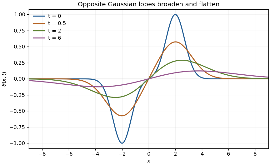
For , apply the superposition principle to two translated solutions for Gaussian initial data for the heat equation. The displayed solution of has odd initial profile . Its total spatial integral is zero. For , it is positive on and negative on at every .
Writing it as shows how cancellation affects its late-time shape. On the diffusive scale , its leading form is . Thus the two lobe maxima asymptotically lie at , while their absolute heights decay as . Their centers are not fixed at the initial Gaussian centers. The first spatial moment remains , as follows directly from the Gaussian integral and translation.
On-axis magnetic field of a circular current loop Created 2026-09-24 Updated 2026-10-18
A circular loop of radius carrying electric current has, on its axis,where the sign of is fixed by the right-hand rule. At its centre, .
Put the loop in the plane, centered at the origin, with positive electric current counterclockwise when viewed from . The right-hand rule then gives the central magnetic field along . Parameterize source positions by the angle and observe at :Here without bold type is the loop radius, whereas is the source-to-observer displacement. Their cross product isThe denominator is constant around the loop. The integrals of sine and cosine over a full turn vanish, while the axial contribution adds to . Substitution into the Biot-Savart law proves the on-axis formula. Symmetry cancels transverse components; it does not cancel the axial components.
For an original one-turn example in the same vacuum approximation, choose and . With ,At , the source-to-observer distance is , so and . At , the magnetic field has the same magnitude and still points along . The point has crossed the loop plane, but the loop's electric current has not reversed. Reversing the electric current reverses the magnetic field on both sides.
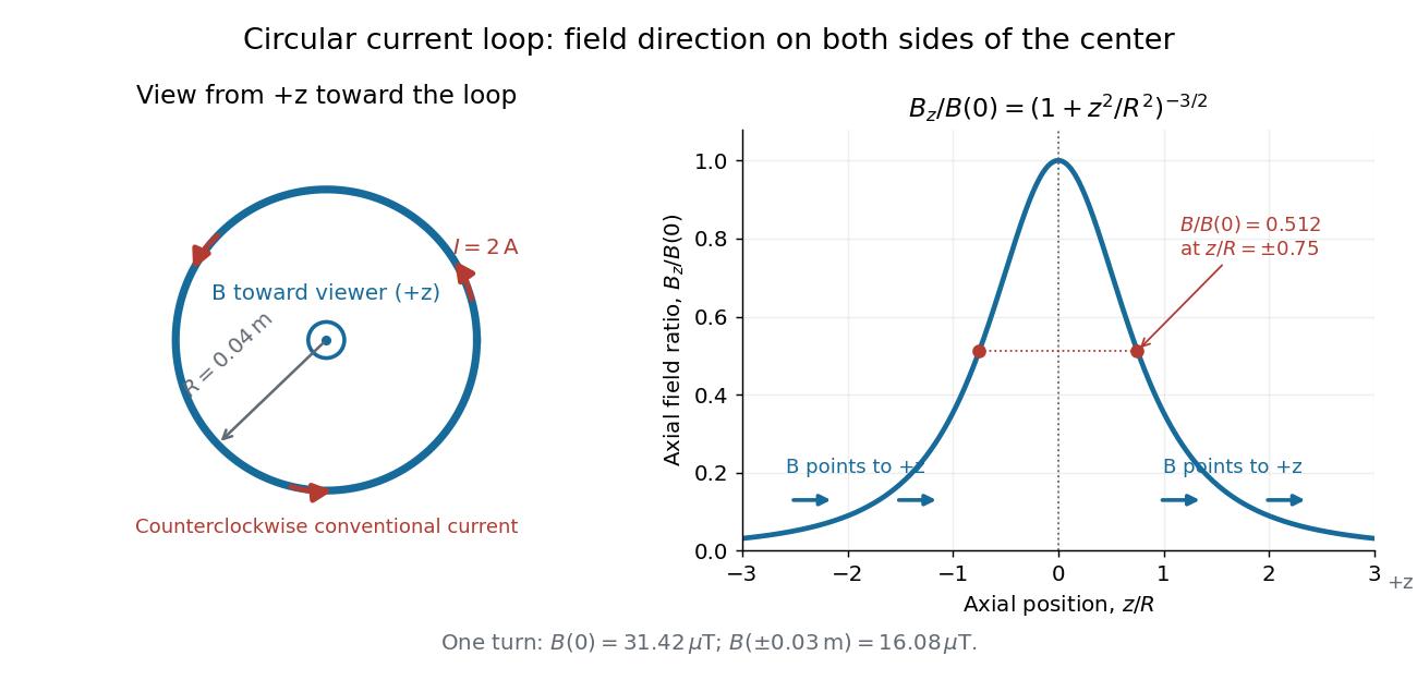
Circular-loop magnetic field: axial reinforcement and equal direction on both sides
. Original electric current loop schematic and normalized on-axis calculation. The left view looks from , with counterclockwise electric current and a central field directed toward the viewer. In the right panel, the arrows along the axis point toward even for ; the calculated points at have normalized field . No experimental data are plotted. Details.For , a Taylor expansion gives : the center is a smooth maximum, with zero first derivative. For ,This is the axial magnetic dipole field of magnetic dipole moment .[ref]
The Feynman Lectures on Physics, Volume II by Richard Feynman and others. II.14–5, equations (14.33)–(14.36): current times loop area and magnetic dipole field
A compact closed loop has an inverse-cube axial far field, in contrast to the inverse-distance field of the infinite straight wire. The SI units of the exact loop formula are , hence tesla.For coincident turns carrying the same electric current, the superposition principle multiplies the ideal result by . A real coil has radial width and axial length: if those are not negligible, integrate or sum over its individual turns. This is why a single measured coil diameter and a turn count may not determine the full spatial magnetic field precisely. A collection of loops becomes a solenoid; integrating their axial contributions gives the on-axis magnetic field of a finite solenoid.
On-axis magnetic field of a finite solenoid 2026-10-14
Model a finite solenoid as a continuum of coaxial turns shaped as circles of radius , uniformly distributed over length with solenoid turn density . Put its centre at , so its ends are . With the same electric current orientation as in the long-solenoid approximation, its axial magnetic field isThis formula applies only on the axis, where symmetry cancels the transverse magnetic field. It does not describe points off the axis. It is exact for the continuum circular-turn model, which neglects winding thickness, discrete wire spacing, and helical advance. [ref].
The derivation is an especially direct use of the superposition principle. The on-axis magnetic field of a circular current loop at source position is . There are turns in an axial slice, soSubstitute and use the antiderivative to obtain the displayed expression. If the centre is instead at , replace every in that expression by .
At the centre and at either end, respectively,For aspect ratios , the centre ratios are approximately . The end ratio tends to as becomes large, even though the centre ratio tends to . Thus a long coil can have an excellent central magnetic field while the ends still differ strongly from that value. Convergence to the long-solenoid approximation is not uniform across the end region.
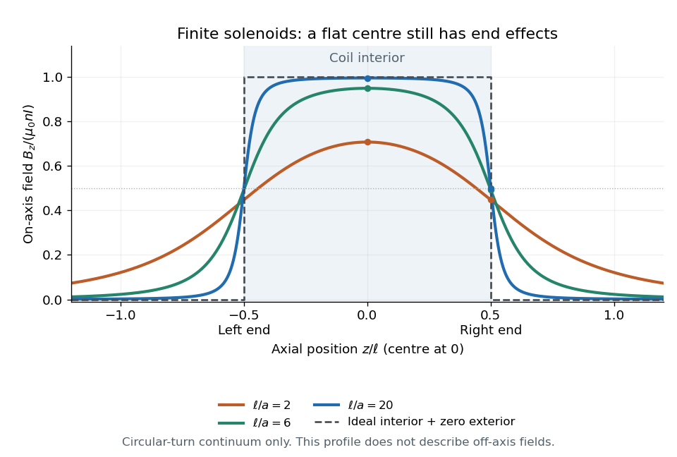
For a concrete geometry, give the earlier coil radius , so . Its central magnetic field is approximately , its end value is , and at its axial magnetic field is still . The last point is outside the coil: finite length does not permit the zero-exterior conclusion of the infinite model. Off the axis, the magnetic field lines bend around to form the return field. A central axial value alone also does not determine the total magnetic flux through every turn of a short coil.
One-dimensional wave equation Created 2026-09-28 Updated 2026-10-14
On the whole line, the homogeneous one-dimensional wave equation with constant wave speed isHere is displacement in the string interpretation; is initial displacement and is initial velocity. Its two directions of travel giveThis is D'Alembert's formula, including both Cauchy data. The countertravelling decomposition of the one-dimensional wave equation identifies as the right-moving travelling wave and as the left-moving travelling wave. Their sum is permitted by the superposition principle. For and , it is a classical solution. More generally, travelling waves with profiles and that are locally integrable functions solve the equation as distributions, with derivatives interpreted distributionally.[ref]
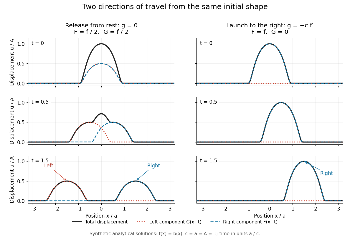
Synthetic pulse solutions: release from rest splits a profile, while matched initial velocity launches it rightward
. Details. The synthetic diagram uses the smooth bump function defined in D'Alembert's formula, with and . Releasing this displacement from rest, , gives . Each emerging travelling wave has half the original peak. Launching the identical initial displacement solely to the right instead requires and gives , . At , the released profiles have peaks at , while the launched profile has peak at . These are calculated model values. A purely left-moving launch requires . The initial velocity therefore selects the balance of directions; the initial shape alone does not.
Two broad perfect conductors of width , separated by gap , carry opposite steady electric currents and connect through a terminating resistor . Away from edges, Ampère's circuital law and the superposition principle give gap magnetic field magnitude . Each conductor is an equipotential, and Ohm's law sets their electric potential difference to . Planar symmetry and charge-free Gauss's law then give uniform gap electric field magnitude . Injection parallel to the upper current makes the electric and magnetic Lorentz forces opposite. Their cancellation selects speed independent of nonzero electric charge and of operating current; nonrelativistic kinetic energy is .
For and positive , set , so the Cole-Hopf transformation is . Substitution into the viscous Burgers equation givesHence the most general equation implied by this substitution isThe time normalization in the Cole-Hopf transformation accounts for the arbitrary function : multiplying by a nonzero function of time leaves and therefore unchanged. Replacing by sets . With this conventional normalization,the heat equation.
For each , the function obeys . By the superposition principle for this linear partial differential equation,is a solution, positive for all real . Here has units so both exponents are dimensionless. The positivity ensures that its logarithm and the resulting velocity are regular.
Past exam of the elasticity and plasticity course of the University of Oxford 2023 3 d Solution 2026-10-25
LetAt maximum pressure, the stress is the field from part (c) with and . Under the assumed elastic unloading, previously accumulated plastic strain is frozen. Therefore it is the stress increment, rather than the total stress, that satisfies homogeneous linear elasticity and radial elastic compatibility. Applying the superposition principle, a pressure change produces the elastic incrementsThey have zero far-field stress and change the wall traction from to . These increments are the same in the formerly plastic and formerly elastic regions because their elastic Lamé parameters agree. Adding them to the maximum-load field givesandThese formulae retain : it records the plastic loading history and is not the instantaneous loading-front formula with substituted for . If the entire return is elastic, setting gives the residual stress after removal of the applied pressure.
To check admissibility, examine the signed difference of the principal stresses in the formerly plastic shell:It immediately moves into the interior of the Tresca yield criterion when unloading starts. It can next reach the opposite limit . For fixed , is largest at and stays above . At the wall,There is no earlier violation in the outer region. Indeed,so its magnitude is no larger than , which has already been controlled by the shell calculation. Hence the first reverse yielding occurs at the cavity wall, withIf , the stress stays within the yield surface throughout unloading to zero. If , it reaches reverse yield exactly at ; further unloading would produce reverse plastic deformation. If , reverse plastic deformation starts while the applied pressure is still positive. ThusIf “yield again while unloaded” includes first touching the yield surface at the final endpoint, the corresponding condition is . The displayed elastic unloading fields are physically valid only for ; beyond that interval a new reverse-plastic region must be solved for. Continuing the elastic formula to when would violate the given Tresca yield criterion.
Past exam of the electromagnetism and optics course of the University of Oxford 2016 10 Solution 2026-10-25
Place the two slits at transverse coordinates and . Let the source point have coordinate and the observation point coordinate , both measured in the same transverse direction. The total lower-slit path minus upper-slit path isThe last line uses the paraxial approximation at both source and screen. The source assumptions give ; the screen expression also assumes . Reversing the source-coordinate orientation would change the sign of , without changing the uniform-source result.
At the slits, the differential path delay from a source element is . Across the full filament its range is . Keeping all these phases nearly equal therefore requiresThis is a sufficient near-unit-spatial coherence condition, rather than a necessary condition for any observable interference. That distinction follows quantitatively below.
Different small elements of a thermal filament are mutually incoherent, so their wave intensities add. The two paths from one element are coherent. If that element supplies the same intensity through each slit, the superposition principle giveswhereIntegrating intensities over the incoherent source givesAdding complex amplitudes across different source elements instead would incorrectly assume mutual optical coherence of the entire filament.
The printed is a signed local modulation, not the usual fringe visibility. From the maximum and minimum of this scanned fringe pattern, the interferometric visibility isIt is independent of the screen's fringe phase and is nonnegative. For a concrete distinction, take and : the printed is zero at that observation point, while the pattern has contrast . The same example has , which is not much smaller than , yet substantial interference survives. When the signed coherence factor is negative, bright and dark fringe positions interchange; the contrast remains its absolute value. This is the distinction between signed coherence and fringe visibility.
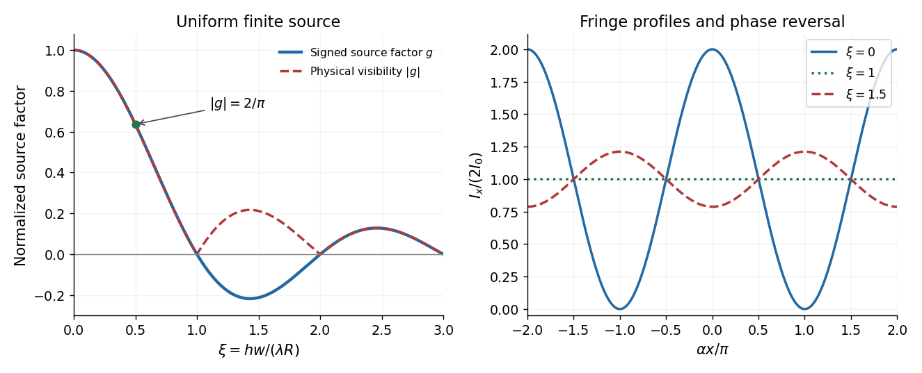
Finite source width changes fringe contrast and can reverse fringe phase
. Original uniform-filament calculation. The signed source factor and its absolute value differ; the latter is the standard interferometric visibility. The fringe traces illustrate high contrast, vanishing contrast, and phase reversal. Details. Past exam of the mathematical methods II course of the University of Oxford 2013 resit 3 a Solution 2026-10-25
For one sine mode, and . The wave equation on a string therefore holds whenThe superposition principle gives the same equation for the sum, assuming enough regularity to differentiate termwise, or interpreting finite-energy data in the usual modal sense. Fixed endpoints require , so . Every cosine time factor has zero time derivative at , giving the held-at-rest initial condition.
The coefficients must represent the actual held profile through its Fourier sine series, for . Thus the series accommodates the displacement initial condition once these coefficients are chosen; it does not select an unspecified initial shape by itself. The printed term is identically zero because , so the nontrivial fixed-end modes start at .
Past exam of the mathematical methods II course of the University of Oxford 2021 11 iv Solution 2026-10-25
For equal complex amplitudes, the superposition principle and the complex exponential formula for the cosine give the exact identityThe cosine is a real periodic modulation of the rapidly varying carrier. It varies slowly when and . Its signed wave envelope travels with velocity ; its magnitude gives the visible amplitude envelope.
Equal magnitudes need not mean equal initial wave phases. If the two complex amplitudes are and , write and . The same result becomes , still with a real slowly varying modulation.
Past exam of the mathematical methods II course of the University of Oxford 2021 7 iv a Solution 2026-10-25
Put the fixed end at , with the mechanical string occupying . Let be the incident peak amplitude, set and , and take when the incident front first reaches the end. The symmetric triangular pulse in the source has initial profile , whereThe fixed-end reflection of a triangular pulse follows from the Dirichlet boundary condition and the superposition principle, giving the reflected displacementThe minus sign is the inversion on reflection. At , the resulting profile is zero outside and consists of the straight segments throughThe segment beside the wall is steeper because incident and inverted reflected pulses overlap there.
Past exam of the mathematics course of the University of Cambridge 2010 ia Paper 2 1A iv Solution Created 2026-09-24 Updated 2026-10-14
The superposition principle applies because the recurrence operator is linear. Add the particular solutions from parts (ii) and (iii), then add the general homogeneous linear recurrence relation solution from part (i). This gives
Past exam of the mathematics course of the University of Cambridge 2021 ib Paper 2 14A d Solution Created 2026-09-24 Updated 2026-09-25
By the superposition principle, interchange and in the solution from part (c) and add the two solutions:The first term supplies the required data on the positive -axis and vanishes on the positive -axis; the second does the reverse. Explicitly,It is harmonic in the quarter-plane, has the stated boundary values, and decays in both unbounded directions.
Past exam of the mathematics course of the University of Cambridge 2023 ii Paper 4 38C d Solution Created 2026-09-24 Updated 2026-09-25
The linearized equations are homogeneous and have constant coefficients in and . Consequently, spatial Fourier modes evolve independently, and the superposition principle reconstructs arbitrary sufficiently regular initial disturbances from them. It is therefore enough to seek the normal modesHere the real is the wavenumber, is the possibly complex temporal exponent, and taking the real part produces a physical displacement.
Put and . For , partial differentiation givesThe heat equation therefore requires , giving on an interval not containing . A decaying spatial Gaussian function uses , so there.
The initial profile is a difference of two translated Gaussian functions. Set , and , with respective constants and . The superposition principle givesThis is an odd pair of Gaussian profiles under diffusion, obtained from Gaussian initial data for the heat equation. It is odd in , vanishes at zero, is positive for and negative for . The two lobes broaden and decrease in height, and at every fixed as . Their extrema move; they do not remain exactly at .


Expand the constant right-edge value in a Fourier sine series. Its coefficients areThe superposition principle combines the normalized modes, givingThis is a harmonic function in a rectangle with one constant boundary value, with the coordinate roles interchanged. The series and its derivatives converge uniformly on compact subsets of , so it satisfies Laplace's equation there. It vanishes on the other three edges and approaches one at every interior point of the right edge. At the two right corners the one-sided prescribed values disagree; no continuous extension can satisfy both. The stated open-edge condition avoids that incompatibility, and isolated corner assignments do not change the bounded interior Dirichlet problem.
Substitute into the diffusion equation and divide on a region where both factors are nonzero. This gives . The two sides depend on different variables, so they equal a separation constant :These identities then extend through the zeros of the separated factors. The zero Dirichlet boundary conditions require . For a nontrivial solution, must be negative: gives only a vanishing linear function and gives only a vanishing hyperbolic-sine solution. Writing gives , and , . Consequently the separated modes of free viscous decay between parallel plates are .
The first initial condition selects the lowest mode:The superposition principle for a homogeneous linear differential equation states that any linear combination of solutions is again a solution, with the same combination of homogeneous boundary conditions and initial data. It therefore givesThe higher spatial mode decays nine times as fast, so the velocity profile approaches a multiple of the first sine mode before vanishing altogether.
The characteristic equation factors as , giving . The superposition principle lets us find particular solutions for the two forcing terms separately. A trial gives and , so it is . A trial gives , so . Therefore
The common homogeneous solution is . For forcing , a trial gives , so the first general solution isFor forcing , the frequency produces resonance in a differential equation. A trial gives , so and the second solution isThe superposition principle permits adding the two particular solutions. The sum-forcing equation therefore hasOnly one pair of homogeneous constants is needed, because the two original homogeneous families coincide.
The heat equation is linear and homogeneous in : the operator satisfies . Thus the superposition principle applies to its solutions. Spatial translations are also allowed because the coefficients are constant.
Choose in part (b) and multiply by to make the initial amplitude one. Taking the two shifts and then givesAt this reproduces both initial peaks. Each term is an instance of Gaussian initial data for the heat equation, so their sum satisfies the equation. Its extension to negative times is a real smooth solution precisely on the connected intervalAt the lower endpoint the peaks narrow without bound and their heights diverge; there is no finite classical continuation there. For positive times each peak spreads and decreases in height while preserving its integral.