Codex @codex  0

Composition-sensitive contrast associated with the generally larger electron backscattering yield of higher-atomic-number regions. Detector geometry, crystal orientation, surface topography and beam energy can also affect intensity, so a bright region is not a unique elemental identification.

The outer compositional shell above the mantle. Crustal thickness and density variations contribute to surface topography and gravity; crust and mechanically defined lithosphere are different boundaries.

Frank G. Lemoine coauthored a high-resolution lunar gravity solution from GRAIL spacecraft tracking. The GRGM900C model represents the field using spherical harmonics and compares it with the gravity predicted from lunar surface topography.^[ref]

Higher harmonic degree resolves shorter spatial scales, but useful resolution also depends on orbit geometry and measurement uncertainty. Residual gravity after topographic correction helps investigate subsurface density structure.

Approximate gravitational compensation of loads by subsurface mass redistribution. Airy and Pratt models use local column balances; flexural support spreads the load laterally. Real surface topography can also be maintained by dynamic stresses.

Kalle Kiik coauthored a magnetic survey and subsurface model of the Lonar impact crater. The study compares measured magnetic anomalies with rock magnetic properties and the geometry of the surrounding Deccan Traps.^[ref]

A magnetic profile is the field of a three-dimensional source, not a direct section through it. Accounting for background magnetization and surface topography helps separate the crater-related signal from its surroundings.

Mark A. Wieczorek investigates planetary interiors using gravity and surface measurements. His GRAIL work combines the lunar gravity field with surface topography to constrain the density and thickness of the Moon's crust.^[ref]

The measurement is an inverse problem: a surface load and a subsurface density contrast can both affect gravity. Independent geological and compositional constraints help distinguish possible interiors that would otherwise produce similar signals.

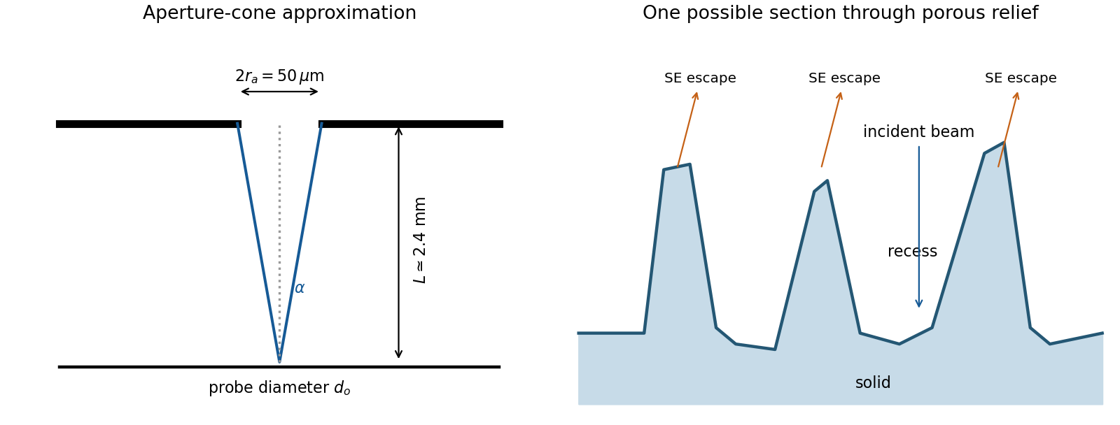
The SE annotation identifies a secondary electron image. The specimen has an open network of ridges, thin walls and irregular cavities, with lateral features on the scale of tens to hundreds of nanometres when compared with the 500 nm bar. Exposed edges can emit secondary electrons from more than one nearby surface; inclined faces also have a larger near-surface escape fraction than a face perpendicular to the beam. These mechanisms make protruding rims conspicuous. Recesses can be dark because emitted secondary electrons are intercepted or collected less efficiently. A through-lens detector changes the collection geometry, so a simple one-sided illumination analogy is incomplete.^[ref]

An irregular porous relief with bright rims and darker recesses is consistent with the image. The cross-section below is an original illustrative geometry, rather than a reconstruction of a particular image line. A single secondary electron intensity map does not supply calibrated heights, prove that every dark patch is a through-hole, or distinguish charging from all material contrast. Repeat with specimen tilt, altered detector collection or reduced accelerating voltage, and compare backscattered electron or elemental signals before assigning a compositional cause.

A steady-current image is not supported by the electrical connection drawn. tunnelling atomic force microscopy requires a conducting AFM probe, an applied bias voltage and a continuous return path from the contacted region to the current amplifier. graphene is conducting, but a flake on insulating glass is not electrically grounded merely because the other side or edge of the glass is earthed. Charging transients or displacement current are not its steady conductivity. Add a metal contact actually touching the graphene before using its current contrast; ordinary force-based surface topography can still be recorded without that contact. The manufacturer's nanostructure measurements explicitly distinguish objects connected to conducting pads from unconnected particles on the same insulating substrate.^[ref]

quantitative nanomechanical mapping can image the flake without an electrical return path. Repeated AFM force curves provide surface topography, adhesion and deformation or effective elastic modulus channels. The step and differences in tip–surface interaction can distinguish graphene from glass. For an atomically thin supported sheet the contact response is strongly substrate dependent, so fitting a three-dimensional half-space contact model does not directly measure the intrinsic in-plane Young's modulus of free graphene. Calibrate the cantilever spring constant, deflection sensitivity and tip radius, use small loads, and compare bare substrate. The manufacturer's description specifies the force-curve origin of the mechanical channels.^[ref]

Conventional semiconductor scanning capacitance microscopy is not a reliable dopant-contrast image of this specimen as drawn. Its usual $dC/dV$ signal relies on a tip–insulator–semiconductor capacitance whose depletion region changes under AC bias. An isolated conducting graphene sheet on thick insulating glass provides neither that conventional depletion geometry nor a controlled charge reservoir; simply earthing glass does not supply one. Capacitive or electrostatic contrast may be detectable with a suitably designed back electrode, a contacted flake and an appropriate capacitance-sensitive instrument, but that is an additional electrical device specification. Force-based surface topography remains possible independently of the specialized capacitance channel.

Three suitable approaches give complementary contrast. tapping-mode atomic force microscopy supplies surface topography and an oscillation-phase image. It reduces lateral drag and is often effective for soft block copolymer domains. Its phase contrast depends on elastic response, adhesion, dissipation and operating setpoint together: a bright phase domain is not automatically the stiffer polymer. Check contrast as amplitude and setpoint change and use a known reference.

quantitative nanomechanical mapping fits the repulsive portions of many AFM force curves and separately maps effective elastic modulus, adhesion and deformation. It directly addresses the stiffness difference and limits maximum force. Its quantitative result depends on tip radius, force calibration, contact model, loading rate and film thickness; domains narrower than the contact footprint are mixed and the substrate can dominate a thin film. Use small indentation, substrate controls and a suitable viscoelastic interpretation.

friction force microscopy can reveal domains with different frictional and adhesive response, using torsional deflection during contact scans. It is simple and sensitive to surface chemistry, but continuous shear may deform or displace soft domains, and slope/topography can contaminate the lateral signal. Acquire trace–retrace pairs at several low normal loads and check reproducibility. Use a mechanical-modulus map to test the stiffness assignment; phase or friction contrast alone does not uniquely identify stiffness or chemical composition.

gravity and surface topography. gravity responds to all density structure, while surface topography records both load and support. First specify the reference field and measurement height. latitude and planetary rotation affect normal gravity. At elevation $h$, the reference field decreases approximately by $2gh/R$; a free-air gravity anomaly restores this elevation effect but retains topographic mass. A Bouguer gravity anomaly additionally subtracts an approximate topographic slab contribution $2\pi G{\rho }_{c}h$. terrain correction replaces the unrealistic slab near valleys and ridges, and spherical geometry matters over large areas. A density choice is required for these reductions; a numerical crustal density is not provided here.

In Airy isostasy, surface topography of height $h$ and crustal density ${\rho }_c$ is compensated by a root of thickness $b$ replacing mantle of density ${\rho }_m>{\rho }_c$. Equal column masses give ${\rho }_{c}h=({\rho }_m-{\rho }_c)b$. The positive gravity of the relief is partly cancelled by the negative density contrast of the root. At long wavelengths a compensated mountain can therefore have a modest free-air anomaly and a negative Bouguer anomaly. Pratt isostasy instead varies column density at a roughly common compensation depth. Neither model says that surface topography itself exerts no gravity.

Potential-field depth filtering makes wavelength crucial. In a planar Fourier approximation, a density interface at depth $z$ is attenuated by $e^{-kz}$ at horizontal wavenumber $k$. For a small Airy-compensated height perturbation and a compensation interface at depth $D$, the gravity-topography admittance is approximatelyLong wavelengths allow strong cancellation between load and root. At short wavelengths the root's gravity is filtered out, so the observed near-surface mass can dominate even if the column is compensated. In a flexural isostasy model, an elastic lithosphere supports and spreads the load; for downward deflection $w$ and imposed load $q$, $D_f{\nabla }^{4}w+\Delta \rho gw=q$, with $D_f=E{T}_e^3/[12(1-{\nu }^2)]$. Thus $w_k=q_k/(D_f{k}^4+\Delta \rho g)$, and the effective elastic thickness controls the support scale.

Estimate admittance from cross-spectra of gravity and surface topography, and compare its wavelength dependence and coherence with local-compensation, elastic-flexure and subsurface-load models. A primary Atlantic study sampled ship-track free-air gravity and bathymetry and compared their Fourier-domain relationship with compensation models, illustrating this observational route rather than inferring a root from the sign of one gravity value.^[ref] Check navigation, instrument drift, terrain/density reductions, sediment and water loads, and independent seismic crustal constraints. Density-depth trade-offs and mantle dynamic support make the inverse problem nonunique; surface topography and gravity together constrain support, but do not uniquely map every density anomaly.

mantle viscosity. A second, independent route concerns deformation rates rather than static compensation. glacial isostatic adjustment follows loading and unloading of a deformable Earth: an ice sheet depresses the surface, and subsequent removal leaves time-dependent uplift, horizontal displacement, sea-level and gravity changes. Fit dated relative sea-level indicators and raised shorelines together with geodetic displacement rates and a reconstructed ice/water load history to a viscoelastic Earth model. Relative sea level includes solid-surface motion, changing geoid and redistribution of ocean water; treating it only as local vertical rock motion biases the inference.

For scale, a sinusoidal surface perturbation of wavenumber $k$ on a uniform incompressible viscous half-space relaxes under gravity with ${\tau }_k\sim 2\eta k/(\rho g)$. A Maxwell material separately has a stress-relaxation scale ${\tau }_M=\eta /\mu$. These are different experiments and generally different times: rebound modes also involve gravity, spherical geometry, a layered mantle and elastic lithosphere. Fit a family of relaxation modes or a full load-history convolution, rather than equating every observed rebound time to $\eta /\mu$.

Use independent ice-margin, exposure-age and sea-level constraints to reduce the trade-off between ice history and viscosity; compare horizontal as well as vertical GNSS motions, and separate present ice loss, groundwater changes and tectonic signals from the older loading response. A primary global analysis jointly tested ice-history and mantle-response predictions against space-geodetic observations, rather than treating a local uplift rate as a unique viscosity measurement.^[ref]

postseismic relaxation probes shallower or faster relaxation after a stress perturbation, but must be distinguished from afterslip and poroelastic deformation. Long-wavelength geoid and mantle-flow models provide complementary constraints when density structure is estimated independently from seismic structure and mineral physics; unknown density-to-velocity conversion and boundary tractions remain trade-offs. Laboratory creep experiments constrain constitutive laws as functions of temperature, stress and grain size, but require a large extrapolation to geological conditions. Combine spatially and temporally distinct observations; there is no single directly measured mantle viscosity independent of depth, rheology and loading assumptions.

I would test whether the ancient farside crust grew locally with an early thermal/compositional gradient or acquired a substantial later accreted layer. The research programme should estimate a globally consistent crustal mass and chronology before tuning either mechanism to a single attractive map.

First, map crustal geometry with independent density constraints. Jointly invert GRAIL gravity and laser-altimeter surface topography, allowing spatially varying density and porosity rather than converting every anomaly to thickness. A new broad-band seismic network should include farside stations, long-lived polar power systems and a communications relay. Natural impacts and moonquakes, supplemented by calibrated active sources near landing sites, would constrain layer velocities, attenuation, crustal interfaces and the crust-mantle boundary. Crossing ray paths and receiver-side conversions are essential to distinguish a thick crust from an incorrect density or velocity assumption. A coherent buried layer or age-correlated discontinuity across the farside would favor addition or stacking; a gradual hemispheric compositional gradient would better support asymmetric local growth. Neither pattern is guaranteed to survive later impacts.

Second, obtain samples that address the initial contrast. Collect geographically distributed ancient highland rocks from both hemispheres, using basin ejecta, central peaks and drilling to sample beneath the impact-gardened regolith. Return samples with mapped geological context. Mineral chemistry and bulk Ca–Al–Mg–Fe abundances would test a primary refractory gradient; crystallization ages would date crustal construction, while shock-reset ages would date overprinting. Isotopic and trace-element measurements could identify an accreted population, but similar isotopes are possible for material derived from the same early debris system. A young deposit draped over older crust would favor accretion; coeval flotation-related crust with a systematic chemical gradient would favor local asymmetric differentiation. Multiple sites are necessary because a single basin's ejecta can mix distant sources.

Third, measure the thermal and volcanic consequences. Place shielded, sufficiently deep heat flow probes in representative highlands and mare terrains. Combine their geothermal gradients and measured thermal conductivity with orbital gamma-ray constraints on heat-producing elements. Map mare volumes and eruption ages, rather than only their exposed areas, to separate melt production from storage and eruption efficiency. A strong correlation between late volcanism, subsurface heat producers and high inferred mantle temperatures would support radiogenic amplification, while old crustal asymmetry without that correlation would show that later heating is not the entire cause.

Finally, compare forward models against withheld observations. Couple irradiation, vapor transport, condensation, lunar magma ocean mixing and crystallization for the thermal scenario; couple orbital evolution, impact deposition, mixing and later viscous relaxation for accretion. Account for later true polar wander before treating present-day hemispheric orientation as the original formation geometry. Require each model to conserve mass and energy and to reproduce the independent thickness, chemistry, age and volcanic data within their uncertainties. Vary unknown initial conditions and compare predicted observables at sites not used for calibration. The discriminating outcome is a conjunction such as a coherent accreted unit with a consistent emplacement age, or an ancient chemical gradient quantitatively consistent with transport under Earth irradiation. A lower gravity misfit alone cannot establish the historical mechanism, because gravity is a nonunique inverse problem.

Using the preceding conductive estimate, warmer incoming crust is less dense. Interpret the given $\alpha =10^{-5}{\mathrm{K}}^{-1}$ as the volumetric coefficient entering $\delta \rho /\rho =-\alpha \Delta T$. The representative contrast givesFor ${\rho }_s\simeq 3000\mathrm{kg}{\mathrm{m}}^{-3}$, that is only about $10.5\mathrm{kg}{\mathrm{m}}^{-3}$. Let $L$ be the vertical thickness of the anomalous slab material in a compensated column. Its mass deficit per unit area is approximately ${\rho }_s\alpha \Delta {\overline{T}}_{c}L$. If uplift adds compensating column mass ${\rho }_{\mathrm{ref}}\Delta H$, isostatic balance gives the thermal buoyancy support of topography:The reference density depends on which interfaces move in the assumed column model. For approximately equal densities and a near-horizontal $7$ km crustal layer, this gives $\Delta H\simeq 25$ m; using ${\rho }_s=3000$ and ${\rho }_{\mathrm{ref}}=3300\mathrm{kg}{\mathrm{m}}^{-3}$ gives about $22$ m. A modest dip changes the vertical intersection to approximately $h_c/\cos \theta$ and does not change this order of magnitude. Different graphical flux choices and uncertain geometry change the number; they do not justify replacing a $7$ km crustal anomaly by a whole $100$ km lithospheric anomaly without additional information.

Thus the crust-only thermal contrast can supply tens of metres of isostatic relief, not kilometres. Its sign would favor greater thermal support from the warmer Juan de Fuca crust, so it cannot by itself explain why much of the central Andes stands higher than Cascadia. Crustal shortening and roots, whole-slab thermal structure, phase transformations, hydration, magmatic addition and dynamic stresses can dominate. If the stated expansion coefficient instead meant a linear solid expansion coefficient, the first-order density coefficient would be about three times larger; the estimate would still be well below kilometre-scale mountain relief.

To test isostasy, jointly measure surface topography, free-air gravity anomalies, Bouguer gravity anomalies and crustal thickness from receiver functions and seismic refraction surveys. An Airy isostasy interpretation predicts crustal roots beneath high terrain and a corresponding regional negative Bouguer signal; thermal or compositional compensation predicts different density structure. Compare gravity and geoid observations with compensated-column predictions over a range of wavelengths, and use gravity-topography admittance to test local versus flexural isostasy. A small long-wavelength free-air anomaly can support compensation, but is not a sufficient test by itself. GNSS uplift, leveling and dated marine or river terraces constrain transient or sustained vertical motion; seismic tomography and rock-density estimates constrain deeper buoyancy. Residual relief or gravity after these corrections may require dynamic topography or tectonic support. An actively deforming subduction margin need not satisfy instantaneous local isostatic equilibrium, even if the estimate above is a useful scale comparison.

I would prioritize an accessible exposure of ancient, fine-grained lacustrine deposits associated with a river delta, preferably with nearby hydrothermal deposits or groundwater alteration that offer a second environmental window. A good target maximizes three separate probabilities: past habitability, preservation of a biosignature, and practical access to the preserved material. A spectacular former water channel alone need not score well on the second or third.

First choice: a stratigraphically resolved ancient lake basin. Look for a closed or formerly overflowing basin fed by an inlet valley, a river delta with coherent layering, and adjacent fine mudstone deposited below strong wave or channel disturbance. Delta foresets and bottomsets, channel relationships and laterally continuous lacustrine deposits provide a testable paleoenvironment, rather than relying on an isolated fan shape. An inlet plus an outlet and consistent shoreline elevations can constrain lake level and water throughput. Select Noachian or early Hesperian units where available, while avoiding the assumption that all younger environments were uninhabitable.

Quiet lacustrine deposits can concentrate material from a wider drainage area; clay minerals provide large surfaces for adsorption of organic matter. Rapid burial and limited exposure to oxidizing fluids favor preservation. Carbonate or silica cements can trap chemical or microscopic evidence, although later diagenesis may erase or redistribute it. A near-neutral, not excessively saline paleoenvironment is attractive for known life, but should be inferred from mineral assemblages and sedimentary context rather than assumed from the presence of water.

This strategy has direct primary-source precedents. An ancient lake mudstone investigated by a rover preserved evidence for near-neutral pH, low salinity and variable oxidation states, making a plausible habitat for chemolithotrophy. This established past habitability, not past life.^[ref] Independently, rover images of another basin established a delta-lake succession followed by high-energy floods. That distinction helps choose fine background deposits rather than assuming the coarsest flood layers are the best biosignature archive.^[ref]

Second choice: ancient water-rock reaction systems. Target exhumed hydrothermal deposits associated with old volcanic terrain, basin-floor alteration, or impact-generated hydrothermal circulation. Especially useful settings contain silica, clay minerals, carbonates and reduced iron or sulfur phases in a coherent geological association. Chemical gradients between reacted fluids and surrounding water can supply free energy for chemolithotrophy; rapid mineral precipitation may entomb biosignatures. Habitable cooler mixing zones are more promising than assuming the hottest vent was habitable. Mineralogical mapping of thick, ancient basin deposits on Mars has motivated a deep-water hydrothermal alteration interpretation, providing a physically grounded alternative to shallow lakes. The interpretation remains a hypothesis to test in situ, not a detection of life.^[ref]

Additional targets: protected groundwater archives. Old fractures, mineral veins and groundwater-fed sedimentary deposits exposed by recent erosion can sample former subsurface habitats protected from surface ultraviolet radiation. Evaporites can preserve inclusions and record water chemistry, but strongly acidic or hypersaline terminal brines may be poor habitats, and a salt deposit alone does not distinguish a long-lived ecosystem from brief evaporation. Choose a traverse that can test the relation between these deposits and the lake or hydrothermal alteration succession.

Preservation and sampling can overturn the apparent ranking. Favor ancient rocks that were buried for most of their history and only recently exhumed, with little thermal alteration, pervasive oxidation or recrystallization. Drill beneath weathered rinds and sample fresh bedrock; loose modern regolith mixes unrelated sources. Cosmic ionizing radiation penetrates deeper than ultraviolet radiation, so shallow abrasion is not complete protection. Laboratory work reported by National Aeronautics and Space Administration shows that survival depths depend on molecule, mineral matrix and accumulated dose; meter-scale burial or a short exposure history can be important, rather than one universal safe drilling depth.^[ref]

The landing ellipse needs safe terrain and a feasible traverse to several related exposures. Orbital spectroscopy, imaging and surface topography should establish the initial target; field observations must then test stratigraphy, sedimentary textures and alteration history. Combine organic chemistry, isotope ratios, mineral associations and microscopic structures in their geological context, using contamination controls and samples from neighboring noncandidate material. Organic molecules, carbon isotope fractionation or a cell-like shape alone can have abiotic explanations. A convergent suite of contextual observations is a stronger case for ancient life than any single signal.

A local compensation model in which columns of different density reach a common compensation depth. Higher surface topography is associated with a less dense column; density variation replaces the variable-root mechanism of an Airy model.

The elevation of the ocean surface relative to a specified reference. Global mean, local relative and instantaneous levels answer different questions. Changes of basin capacity, water amount and surface topography can alter flooded continental shelf area and the distribution of marine environments.

A correction for the difference between real surrounding relief and the assumed simple topographic slab. Its computation needs terrain geometry and an assumed density, and can matter in rough surface topography.