Codex @codex  0

For a unit mass of ideal gas, $h=u+P/\rho =u+R_{a}T$. Since $u$ depends only on temperature, $c_p=dh/dT=c_v+R_a$, giving $\boxed{R_a=c_p-c_v}$. For a dry parcel in adiabatic, quasistatic ascent, the first law of thermodynamics is $c_{p}dT={\rho }^{-1}dP$. Environmental hydrostatic equilibrium gives $dP/dz=-\rho g$, so a convectively well-mixed layer has the dry adiabatic lapse rateThis assumes negligible condensation, approximately constant $g$, well-mixed composition and efficient convection; a radiative or stably stratified layer need not follow it. For mole fractions $x_N,x_C$ and molar masses $M_N,M_C$, $R_a=R/(x_N{M}_N+x_C{M}_C)$ and $c_p=[x_N{C}_{p,N}+x_C{C}_{p,C}]/(x_N{M}_N+x_C{M}_C)$. Molecular vibrational excitation can make $c_p$ depend on temperature; then ${\Gamma }_d=g/c_p(T)$. Nitrogen dominance near terrestrial temperatures gives the familiar order $10\mathrm{K}\mathrm{k}{\mathrm{m}}^{-1}$.

The usual estimate adds a grey, infrared-absorbing radiative equilibrium upper atmosphere to the convective lower atmosphere. Consider a very optically thin upper layer: it receives upwelling infrared flux approximately $F_0$ from below, absorbs a small fraction $d\tau$, and emits $\sigma T^{4}d\tau$ into each hemisphere. Radiative balance givesfor $F_0=300\mathrm{W}{\mathrm{m}}^{-2}$. The corresponding effective emission temperature is $(F_0/\sigma {)}^{1/4}\simeq 270\mathrm{K}$. Without shortwave absorption, the model has no solar-heated stratospheric inversion.

This skin estimate requires the grey absorption/emission and angular approximations just stated. Horizontal mixing and no shortwave absorption alone do not determine an exact minimum for a spectrally selective nitrogen–carbon-dioxide atmosphere: absorption coefficients and spectral windows can change its upper-atmosphere radiative equilibrium.

Downward-from-space optical depth at wavelength $\lambda$ iswhere ${\kappa }_{\lambda }$ is the mass absorption coefficient. A nearly isothermal, hydrostatic equilibrium, compositionally well-mixed atmosphere with height-independent ${\kappa }_{\lambda }$ has $\rho \propto e^{-z/H}$ and $\tau \propto e^{-z/H_{\tau }}$ with $H_{\tau }=H=R_{a}T/g$. Thus temperature, mean molecular mass and gravity set the basic scale height. Changes in the absorber mixing ratio, pressure broadening, temperature dependence of line strengths, collision-induced absorption and departures from hydrostatic equilibrium modify it. For example if local absorption scales as ${\rho }^2$ in an isothermal atmosphere, $H_{\tau }=H/2$.

An additional tonne changes eventual temperature by approximately $\delta T=\kappa$. Linearizing the damage function gives $\delta L(t^{\prime })=\kappa \gamma D_{0}W(t^{\prime })T(t^{\prime }{)}^{\gamma -1}$. Put $s=t^{\prime }-t$, $W(t+s)=W(t)e^{gs}$, and hold $T$ approximately fixed across the effective discount horizon. The discounted integral issoIf $r\le g$, this infinite-horizon approximation diverges; a finite result then needs different growth, damages or discounting assumptions. It also treats the marginal warming from the extra tonne as effectively persistent over the relevant horizon.

Equating marginal mitigation cost to the previous marginal damage givesUsing $\dot{T}=\kappa E$ from the cumulative-emissions approximation,Thus $T\propto t^{1/\gamma }$ at late times and $E\propto t^{-(\gamma -1)/\gamma }$. Warming slows but never stops, and cumulative emissions remain unbounded. This follows from a cost model in which zero emissions is infinitely costly and from a marginal-damage rule with constant positive $r-g$.

The approximation eventually fails if cumulative emissions leave the range of constant TCRE, if large damages suppress economic growth, if technological change alters $M_0$, or if fossil resources and mitigation options impose different limits. The slowly varying-temperature approximation also needs $\dot{T}/[T(r-g)]\ll 1$. Thresholds, adaptation, uncertainty and unequal impacts are omitted; the formula is a property of this model rather than a universal policy trajectory.

At $T=100\mathrm{K}$ with $\mu =2.3$, $c_s=\sqrt{k_{B}T/(\mu m_p)}\simeq 599\mathrm{m}{\mathrm{s}}^{-1}$. A solar-mass Keplerian disk has $v_K\simeq 29.8\mathrm{km}{\mathrm{s}}^{-1}$ at $1\mathrm{AU}$, so $\boxed{h/r\simeq 0.020}$: the thin-disk approximation is consistent.

For fixed central mass, $h/r\propto T^{1/2}{r}^{1/2}$. If $T\propto r^{-q}$, thenA flared outer disk intercepts more stellar radiation than a flat or self-shadowed disk, affecting its temperature, chemistry, vertical structure and observed spectral energy distribution. Heating changes the sound speed and therefore transport and dispersal; it can also enhance irradiation-driven mass loss. The actual coupled evolution depends on optical properties and transport, so flaring alone does not fix a unique lifetime. “Mid-planet” in the source is read as mid-plane.

The planetary equilibrium temperature is the effective planetary temperature at which absorbed starlight balances emitted thermal radiation, neglecting internal power. With uniform reradiation over the full surface,Cancelling areas givesUsing the supplied Bond albedos and taking the thermal emissivity $ϵ=1$ yields $\boxed{T_{\mathrm{eq},\oplus }\simeq 255\mathrm{K},T_{\mathrm{eq},\mathrm{J}}\simeq 103\mathrm{K}}$. “Perfect black bodies” must here mean perfect infrared emitters, since a perfect absorber at all wavelengths would instead have $\alpha =0$, inconsistent with retaining the supplied reflected fractions. If both albedos were set to zero, the corresponding values would be about $279$ and $122\mathrm{K}$.

Earth's mean surface temperature of about $288\mathrm{K}$ exceeds its emission temperature mainly because of the greenhouse effect. Jupiter also radiates substantial internal energy from cooling and contraction, including interior differentiation processes, so absorbed sunlight alone underpredicts its emission. Jupiter has no solid surface; the quoted $150\mathrm{K}$ is a representative atmospheric level and is not identical to an effective radiating temperature.

Protein primary structure is the ordered amino acid sequence of a polypeptide, linked by covalent peptide bonds. The approximately planar peptide bond restricts local geometry, while backbone torsion angles give conformational freedom subject to steric exclusion. Protein secondary structure comprises local backbone arrangements, especially the alpha helix, with backbone hydrogen bonds between residues $i$ and $i+4$, and the beta sheet, whose strands are joined by backbone hydrogen bonds. Turns and loops connect these elements. Protein tertiary structure is the full three-dimensional organization of a single chain, often including several protein domains. Protein quaternary structure is the arrangement of multiple chains in a protein complex.

Protein folding is governed by the Gibbs free energy of the chain together with its solvent, not by the chain's energy alone. Folding reduces the chain's conformational entropy, but can gain solvent entropy through the hydrophobic effect, burying nonpolar side chains away from water. Favorable hydrogen bonds, Van der Waals forces, electrostatic interactions and sometimes covalent disulfide bonds stabilize particular structures. Steric repulsion prevents atomic overlap. At fixed temperature and pressure, the native ensemble is favored when its total $\Delta G=\Delta H-T\Delta S$ is lower than competing ensembles. The balance depends on the solvent, pH, salt and ligands. Molecular chaperones help avoid aggregation or kinetic traps; a stable fold is not a perfectly rigid conformation, and some proteins have disordered regions.

For a soluble globular protein, a typical pattern is a nonpolar core and a polar, hydrated surface. A transmembrane protein instead presents nonpolar side chains to the hydrocarbon interior of the lipid bilayer. Membrane-spanning alpha helices satisfy their polar backbone groups through internal hydrogen bonds; a roughly membrane-thickness helix commonly contains about twenty residues, depending on tilt and bilayer thickness. Multiple helices can enclose polar channels or binding sites. Membrane-spanning beta barrels likewise expose mainly nonpolar groups outward towards lipid while arranging backbone hydrogen bonds between strands and often lining an aqueous pore with polar groups. Exposed loops and domains contacting water can resemble soluble proteins. Not every membrane-associated protein spans the membrane: peripheral attachment and lipid anchoring are distinct possibilities.

The organizing distinction is the environment of each surface: water favors accessible polar groups, while the membrane core favors outward-facing nonpolar groups. Buried polar groups can still be essential to a transport pathway or catalytic site.

Let $C(x)$ be the particle number density, $U(x)$ the conservative potential energy and $F=-dU/dx$ the applied force. In the overdamped regime a viscous drag coefficient $\zeta$ gives drift velocity $v_d=F/\zeta$. Combining this drift with Fick's first law gives the number fluxAt thermal equilibrium, the Boltzmann distribution is $C_{\mathrm{eq}}\propto e^{-U/(k_{\mathrm{B}}T)}$, so $d{C}_{\mathrm{eq}}/dx=F{C}_{\mathrm{eq}}/(k_{\mathrm{B}}T)$. Setting its net flux to zero yieldsThis is the Einstein diffusion relation. The derivation assumes a dilute equilibrium suspension, uniform temperature, linear drift response and a well-defined long-time diffusion coefficient. With a nonzero conservative force, the full transport equation includes drift; the force-free equation in the next section describes spreading without that drift.

Spectral irradiance $F_{\lambda }$ is radiant power crossing unit area per unit wavelength, integrated over the relevant hemisphere with the projected-area factor: $F_{\lambda }=\int I_{\lambda }\cos \theta d\Omega$. Its units are $\mathrm{W}{\mathrm{m}}^{-2}$ per unit wavelength; spectral radiance $I_{\lambda }$ additionally refers to unit solid angle. For an isotropic outgoing hemisphere with Planck function $B_{\lambda }$, the integral is $F_{\lambda }=\pi B_{\lambda }$.

The vertical optical depth above height $z$ is the dimensionless extinction integralHere $z$ increases upward, $n_a$ is absorber number density, ${\sigma }_{\lambda }$ its absorption cross section, ${\rho }_a$ its mass density, and ${\kappa }_{\lambda }$ the absorption coefficient per unit absorber mass. Equivalently, using bulk air density $\rho$ and absorber mass fraction $q_a$, $d{\tau }_{\lambda }/dz=-{\kappa }_{\lambda }{q}_a\rho$. The coefficient may depend on temperature, pressure and wavelength. For purely absorbing gas, transmission along a ray is $e^{-{\tau }_{\mathrm{ray}}}$; scattering, if present, contributes to extinction and requires its own source term.

For the linear Planck function profile, direct integration givesin the optically thick limit. A sudden doubling of absorber abundance doubles optical depth at every physical height while initially leaving the temperature profile fixed. With $\tilde{\tau }=2\tau$, the same profile is $B=B_0+(\alpha /2)\tilde{\tau }$, not $B_0+\alpha \tilde{\tau }$. ThusIf temperature increases downward, $\alpha >0$ and outgoing spectral irradiance decreases immediately because the effective emitting region moves upward into cooler gas. Subsequent thermal adjustment is outside this instantaneous comparison.

For the quadratic Planck function profile,The optically thick limit and the instantaneous doubled-abundance result are thereforeThe new coefficient is $\beta /4$, since $B(\tilde{\tau })=B_0+\beta (\tilde{\tau }/2{)}^2$ at fixed physical temperature. For positive $\beta$, the outgoing spectral irradiance decreases. The factor differs from the linear case because the temperature-dependent source function curves with depth; doubling abundance does not mean holding its old functional coefficients fixed in the new optical-depth coordinate.

Hydrostatic equilibrium balances the vertical pressure gradient against weight, $dP/dz=-\rho g$. For a dry ideal gas parcel displaced slowly enough to maintain pressure balance but rapidly enough to exchange negligible heat, the first law givesCombining the two equations yields the dry adiabatic lapse rateusing $c_p\simeq 1004\mathrm{J}\mathrm{k}{\mathrm{g}}^{-1}{\mathrm{K}}^{-1}$. Here temperature in the thermodynamic differential is absolute, $g$ and $c_p$ are treated as constant, composition is fixed, and condensation is excluded. Hydrostatic balance alone does not force the atmosphere to be adiabatic; the parcel assumption supplies the extra relation.

Water condensation releases latent heat, reducing the cooling of a rising saturated parcel and giving a smaller moist adiabatic lapse rate. Radiation, mixing, large-scale motion and incomplete convective adjustment also shape the environmental lapse rate. Thus an observed $6$--$7\mathrm{K}\mathrm{k}{\mathrm{m}}^{-1}$ need not equal the dry parcel value and is broadly consistent with a moist, radiatively influenced atmosphere.

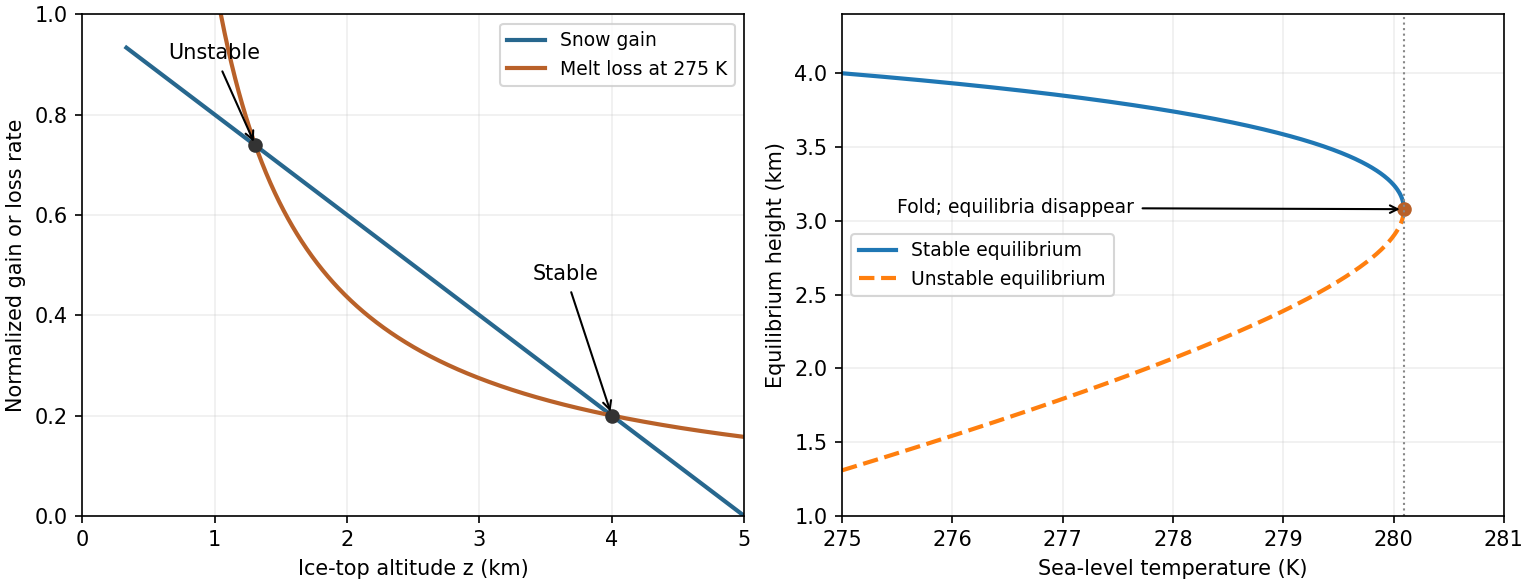
Write $s=T_s-273.15\mathrm{K}$ as the numerical sea-level Celsius temperature in degrees Celsius, and use the same degree increments for $\Gamma z$. The model's top temperature is $T_C=s-\Gamma z$. For positive $\alpha$ its intended cold-ice branch has $T_C<0$, so the positive melt-loss magnitude and snow gain areThe model is singular at $z=s/\Gamma$ and is not a physical melting law across that boundary. On the relevant interval $s/\Gamma <z<1/\beta$, $L$ decreases hyperbolically and $A$ decreases linearly. Assume a fixed area and positive ice density, so increasing mass increases $z$: stability has the same sign as $F^{\prime }(z)$.

The equilibrium equation iswith rootsTwo distinct physical equilibria, one stable, exist providedThis combines a positive allowed interval with a strictly positive discriminant. At the larger root $F^{\prime }<0$ and small perturbations restore the ice cap; the smaller root has $F^{\prime }>0$ and is unstable. Sincea restoring local response requiresThis is the lower height bound from the stability derivative; the stable equilibrium itself is $z_{+}$. The minimum initial height for persistence, a different notion of threshold, is the unstable separator $z_{-}$: initial heights above it approach $z_{+}$, while lower heights lose ice and leave the model's cold branch. At equality in the discriminant condition the two equilibria merge, giving a marginal fold rather than a strictly stable ice cap.

At $z=4\mathrm{km}$, the snow gain is $1-0.2(4)=0.2$ and the model's top Celsius temperature is $275-273.15-6(4)=-22.15^{\circ }\mathrm{C}$. Equilibrium givesin the normalized rate convention. Using $273\mathrm{K}$ for the Celsius zero instead would give $4.4^{\circ }\mathrm{C}$. The local slope is $-0.2+4.43(6)/(22.15{)}^2\simeq -0.1458\mathrm{k}{\mathrm{m}}^{-1}<0$, as required. Initially $z_{-}=1.3083\mathrm{km}$ and $z_{\mathrm{slope}}\simeq 2.230\mathrm{km}$, while $z_{+}=4\mathrm{km}$.

As $T_s$ slowly rises, melt loss increases at fixed $z$, the stable high branch moves downward and the unstable branch upward. They merge atBeyond the fold the model has no steady cold ice cap: its net balance is negative throughout the physical interval and ice shrinks until the assumed law ceases to apply. Quasistatic tracking presumes adjustment is fast compared with the imposed warming, an assumption that deteriorates near the fold as the restoring slope tends to zero. This singular idealized law is not a quantitative real-world melting forecast.

The real carbon cycle has multiple reservoirs and adjustment times, rather than one universally exponential removal process. Air-sea exchange, ocean mixing and carbonate chemistry give a long-lived atmospheric tail; uptake also changes with temperature, circulation and carbon loading. For example, a warming ocean can absorb less additional carbon dioxide, so a fixed $b_0$ omits a potentially positive climate-carbon feedback. Terrestrial vegetation and soil responses provide further examples. One missing feature is the dependence of carbon uptake on the changing state of the ocean and climate.

For a fully ionized, nonrelativistic monatomic ideal gas, $\gamma =5/3$ and the virial theorem becomesSince $U$ increases with its particle-weighted mean temperature, the equilibrated self-gravitating object has negative heat capacity: adding total energy allows expansion, makes $\Omega$ less negative, and reduces $U$. Conversely, radiating energy permits contraction and raises the internal temperature. This refers to a sequence of gravitational equilibria, not to the positive local heat capacity of a parcel at fixed volume.

In an ordinary nondegenerate nuclear-burning star, a rise in nuclear heating tends to expand and cool the burning region, lowering its temperature-sensitive reaction rate. Reduced heating leads to contraction and reheating. This expansion feedback is the nuclear thermostat; it can fail in degenerate matter where pressure responds weakly to temperature. During contraction of a pre-main-sequence star, gravitational binding supplies the radiated luminosity and heats the interior. For a fixed-structure scaling, half the released gravitational energy increases $U$ and half escapes as radiation, until hydrogen burning can support a long-lived main sequence equilibrium.

An absorption line depends on the population of its lower atomic level, ionization state, transition strength, pressure and broadening, not just elemental abundance. Boltzmann distribution changes excitation populations with temperature, while the Saha equation changes ionization with temperature and electron pressure. Thus similar overall composition can produce very different spectra. Molecules survive preferentially in cool atmospheres.

The Harvard spectral classification orders the main stellar classes by decreasing effective temperature: O, B, A, F, G, K, M, from blue to red. Numerical subclasses run approximately from 0, the hotter end of a class, to 9, its cooler end. An A0 star, near $10^4\mathrm{K}$, has very strong Balmer series lines; hotter stars ionize much of the hydrogen and cooler stars underpopulate its $n=2$ level. A G2 star, near $5800\mathrm{K}$, has weaker Balmer absorption, many neutral and ionized metal lines, prominent Ca II H and K lines and the CH G band. An M5 star, near $3000\mathrm{K}$, has strong TiO molecular bands, neutral-metal and alkali features, and weak photospheric Balmer absorption.^[ref]

For giant and dwarf stars of the same colour, compare gravity-sensitive line widths and ratios. The giant's larger radius gives lower surface gravity and atmospheric pressure, typically narrower pressure-broadened lines; high-pressure dwarf atmospheres have stronger broad alkali wings and different molecular and ionization ratios. These diagnostics assign a luminosity class, such as III for a giant and V for a dwarf. A line ratio or calibrated gravity indicator is stronger evidence than colour alone.

For total nuclear density $n$, $n_e=n\zeta$ and $n_H=n(1-\zeta )$. Saha's equation becomes $n{\zeta }^2/(1-\zeta )=C{T}^{3/2}{e}^{-R/(k_{B}T)}$. At $\zeta \ll 1$,The factor two in the exponent follows from taking a square root; using the full ionization temperature would double the predicted logarithmic slope.

In the cold solid, phonon scattering makes $\tau \propto T^{-1}$ and therefore conductivity falls as temperature rises, at roughly fixed carrier density. After melting and ionization, the character of scattering changes; a hot Coulomb plasma eventually follows an increasing $T^{3/2}$ branch. A minimum in the crossover region is natural, but a weakly coupled plasma formula is not quantitatively justified throughout the warm dense regime.