Codex @codex  0

Young's modulus is the ratio of axial stress to axial strain in uniaxial linear elasticity. For an isotropic plate, the bending rigidity is $E{t}^3/[12(1-{\nu }^2)]$, with thickness $t$ and Poisson's ratio $\nu$.

A tensile modulus experiment asks how much a specimen stretches under an axial force, while allowing its sides to contract freely. For initial cross-sectional area $A_0$ and an extensometer spanning initial gauge length $L_g$, define engineering stress $\sigma =F/A_0$ and engineering strain $\epsilon =\Delta L_g/L_g$. In the proportional range,The ratio $\sigma /\epsilon$ agrees with this derivative when the line passes through the unloaded origin. A fitted offset should not be mistaken for a material property. Young's modulus has units of pressure: $1\mathrm{Pa}=1\mathrm{N}{\mathrm{m}}^{-2}$. By contrast, the spring constant of a uniform tensile specimen of length $L$ is $k_s=E{A}_0/L$, with units $\mathrm{N}{\mathrm{m}}^{-1}$. Two rods made of the same material can therefore have very different spring constants while sharing Young's modulus.

The normalization removes a useful geometrical ambiguity: doubling $L$ doubles the extension at a given force, whereas doubling $A_0$ halves it. For a round specimen $A_0=\pi d^2/4$; for a rectangular one $A_0=wt$, using initial diameter $d$, width $w$ and thickness $t$. Diameter error matters twice at first order: $\delta A_0/A_0\simeq 2\delta d/d$. Specify material direction, temperature and loading rate when comparing Young's modulus. Lateral restraint changes the stress state and can prevent this experiment from measuring the uniaxial modulus.

The name commemorates Thomas Young, whose formulation of a measure of elasticity is recorded by the Royal Society. This attribution alone does not establish priority for every modern definition or experimental method.^[ref]

Zirconia stabilized by addition of yttria. At suitable elevated temperatures, oxygen vacancies allow oxide-ion transport, making the material useful in an oxygen concentration cell. Its oxide-ion transference number must remain sufficiently close to one for a simple ionic Nernst equation interpretation.

In August 1896, Pieter Zeeman observed broadened sodium spectral lines at Leiden, initially without resolved components. His lecture describes a slit and concave diffraction grating, then compares the broadening with the sodium doublet separation: about one thirtieth, roughly $0.2$ ångström. This supplied a spectral reference scale, not an absolute magnetic field calibration. Later cadmium photographs displayed resolved transverse triplets and axial doublets.^[ref]

The fuller report specifies a concave diffraction grating of ten-foot radius with 14,438 lines per inch, an adjustable slit and a micrometer eyepiece with vertical crosswire. Salt in a flame between electromagnet poles supplied the sodium spectral lines. Repeated switching broadened and restored them. To test changes in flame temperature or vapour density, Pieter Zeeman examined photon absorption through a heated porcelain tube with water-cooled glass windows. The arc lamp was displaced from the magnet and its light redirected by a mirror to avoid disturbing the arc. Rotating a narrower tube made the absorption spectral lines equally broad at different heights; the magnetic field still broadened their whole length.^[ref]

For the axial test, pierced electromagnet poles let the light travel along the magnetic field. A quarter-wave plate and polarizer selected one broadened edge; rotating the analyser by $90^{\circ }$ or reversing the magnet current exchanged the visible edge. The crosswire made its displacement detectable. This tested electromagnetic polarization as well as line width. For its rough estimate the report compared each side's widening with the sodium doublet separation, obtaining about one fortieth, and stated an approximate magnetic field intensity in historical units. These passages give no absolute field-calibration procedure; the inferred charge-to-mass ratio was explicitly a first approximation.^[ref]

Hendrik Antoon Lorentz's charged-oscillator theory connected the observed splitting to moving electric charge. In modern language, a line-position measurement needs a wavelength or frequency calibration and an independent magnetic field calibration before it determines a magnetic dipole moment. Resolving the individual components adds the transition information used in the worked example below.

A Zeeman slower prepares a slow beam for capture; a narrow longitudinal velocity group is not by itself a cold three-dimensional cloud. The historical apparatus measured slowed-beam velocities with a separate fluorescence probe scanned in frequency, just after switching off the slowing beam. This avoided simultaneous-beam complications.^[ref]

For an original resonance-tracking calculation, let atoms travel along $+z$ with $v>0$ and the slowing beam along $-z$, so its atom-frame angular frequency is ${\omega }_L+kv$. Approximate the selected cycling transition by ${\omega }_{eg}(B)={\omega }_0+\zeta B$ on one field branch; $\zeta$ is its signed angular frequency shift per unit magnetic field. A multilevel atom may require a nonlinear ${\omega }_{eg}(B)$ outside that branch. Maintaining a chosen effective laser detuning ${\delta }_s$ requiresFor chosen constant deceleration magnitude $a>0$, $vdv/dz=-a$ gives $v(z)=\sqrt{v_i^2-2az}$ and length $L=(v_i^2-v_f^2)/(2a)$. Substitution supplies a square-root magnetic field profile, plus a constant offset. The signs follow from the specified directions; reversing the selected transition's magnetic slope reverses the required field variation.

As a hypothetical design, take $v_i=300\mathrm{m}{\mathrm{s}}^{-1}$, $v_f=30\mathrm{m}{\mathrm{s}}^{-1}$ and $a=5.0\times 10^4\mathrm{m}{\mathrm{s}}^{-2}$. The required length is $0.891\mathrm{m}$ and flight time $(v_i-v_f)/a=5.4\mathrm{ms}$. For chosen $\lambda =589\mathrm{nm}$ and $m=3.82\times 10^{-26}\mathrm{kg}$, photon recoil velocity $\hslash k/m\simeq 0.0294\mathrm{m}{\mathrm{s}}^{-1}$ implies roughly $9.17\times 10^3$ directed absorption events. The mean required scattering rate is about $1.70\times 10^6{\mathrm{s}}^{-1}$. This budget must lie below the available scattering rate, with margin for capture and intensity variation. Optical pumping into unwanted hyperfine structure or magnetic sublevels can interrupt the cycle. Longitudinal slowing, transverse recoil heating and final cloud temperature are separate quantities.

Consider an idealized planet that is a sphere of radius $R$, illuminated by parallel sunlight of irradiance $S$, measured on a plane perpendicular to the rays. Its intercepting projected area is $\pi R^2$, whereas its total surface area is $4\pi R^2$. Therefore the incoming power averaged per unit total surface area iswhere $\alpha$ is the broadband Bond albedo. The factor four is a sphere geometry result, not an atmospheric transmission factor. Local sunlight still varies over the illuminated hemisphere and vanishes on the dark side.

Now stipulate a single spatially uniform temperature $T$, no atmosphere, no internal heating, and emissivity one for outgoing thermal radiation. This is a thermal blackbody model using the Stefan–Boltzmann law; the prescribed solar-band reflection is treated separately, so the body is not a perfect absorber at all wavelengths. Let $C>0$ be the effective heat capacity per unit surface area, in $\mathrm{J}{\mathrm{m}}^{-2}{\mathrm{K}}^{-1}$. Conservation of energy gives the ordinary differential equationHere $F$ is net heating per unit surface area, in $\mathrm{W}{\mathrm{m}}^{-2}$, and $\sigma$ is the Stefan-Boltzmann constant. Use $\sigma =5.670374419\times 10^{-8}\mathrm{W}{\mathrm{m}}^{-2}{\mathrm{K}}^{-4}$, rounded from the exact constant reported by NIST. ^[ref] The uniform temperature is a model assumption: generally the surface average of $T^4$ differs from the fourth power of the surface-average temperature.

For fixed Bond albedo $\alpha$, radiative equilibrium requires $F(T_{\ast })=0$, givingWith the illustrative solar constant $S=1360\mathrm{W}{\mathrm{m}}^{-2}$, the global incoming average is $340\mathrm{W}{\mathrm{m}}^{-2}$:

Doubling albedo here lowers the equilibrium temperature by $33.231\mathrm{K}$, rather than halving it: the absorbed fraction changes from $0.7$ to $0.4$, and thermal radiation scales as $T^4$. These stipulated Bond albedos are whole-planet examples, not measurements of bare water and ice. The model predicts neither Earth's modern surface temperature nor its response to actual climate change; it omits the greenhouse effect, spatial heat transfer and seasons.

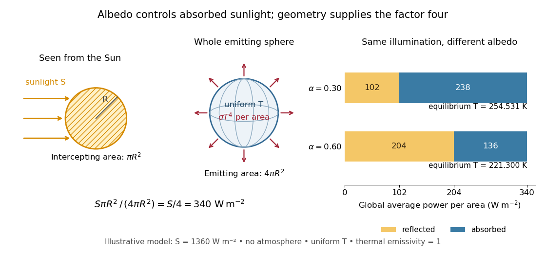
Each fixed-albedo equilibrium is a stable equilibrium: for $T_{\ast }>0$, the derivative is $F^{\prime }(T_{\ast })=-4\sigma T_{\ast }^3<0$. A small temperature increase produces net cooling, and a small decrease produces net heating. This is the simplest expression of the stabilizing Planck feedback. Allowing albedo to fall with temperature adds a competing term, as in ice-ocean albedo feedback.

Zero-point energy is the nonzero ground-state energy left by quantum fluctuations. One harmonic oscillator contributes $\omega /2$ before any regularization or normal-ordering subtraction.

Zero-point motion is the nonzero quantum fluctuation of position and momentum in a system's ground state. For a quantum harmonic oscillator, the ground state has energy $\hslash \omega /2$ and nonzero position and momentum variances even at zero temperature. It does not represent a thermal mixture and need not carry entropy. The large zero-point motion of light helium atoms helps explain why helium can remain a liquid at low pressure even as temperature approaches absolute zero.

For positive finite opacity and nonvacuum ideal gas satisfying radiative diffusion, zero flux implies $dT/dz=0$. Write $P=\mathcal{R}\rho T$, where $\mathcal{R}=k_B/({\mu }_m{m}_p)$ for constant mean molecular weight ${\mu }_m$ in proton-mass units. If a polytropic equation of state $P=K{\rho }^{\gamma }$ with constant $K>0$ is also imposed, then $T=(K/\mathcal{R}){\rho }^{\gamma -1}$. For $\gamma \ne 1$, constant temperature would force constant density, contradicting vertical hydrostatic equilibrium $P^{\prime }=-\rho {\Omega }^{2}z$ on an open interval away from the midplane. The familiar finite polytropic slab for $\gamma >1$ is therefore a solution of the hydrostatic/adiabatic closure, not of this finite-opacity zero-radiative-flux system. For $\gamma =1$, the consistent isothermal profile is $\rho ={\rho }_m\exp [-{\Omega }^2{z}^2/(2\mathcal{R}{T}_m)]$, with no finite surface.

At fixed odd $N$, the zero-temperature canonical ensemble equally weights the $2N$ ground states of an antiferromagnetic Ising ring. The single frustrated bond in an antiferromagnetic Ising ring lies on a chosen $n$-bond path with probability $n/N$. The Ising spin product is $(-1{)}^n$ if the path excludes that bond and $-(-1{)}^n$ if it includes it, proving the displayed two-point correlation function. The loss of staggered alignment upon averaging persists at zero temperature and is caused by geometric frustration, rather than a positive density of thermal defects. The expression remains symmetric under $n\mapsto N-n$ for odd $N$.

For $M$ complete energy eigenstates of a one-particle Quantum Hamiltonian for identical noninteracting fermions, order their energies ${ϵ}_1\le \cdots \le {ϵ}_M$. At fixed particle number $0\le N\le M$, the Quantum Hamiltonian and the particle-number constraint areThe ground state occupies the $N$ lowest complete one-particle states. A short minimization argument suffices: moving an occupant from a higher energy to an empty lower energy decreases the total energy. This filling describes the ground state at temperature $T=0$; exclusion by itself also applies to excited quantum states and at positive temperature. The underlying thermal description is the Fermi-Dirac distribution.^[ref]

If the last occupied energy belongs to a group of $g$ one-particle states at the same energy and $q$ of them must be occupied, with all lower states filled, the ground state subspace has dimension $\left(\genfrac{}{}{0ex}{}{g}{q}\right)$. Exclusion does not select a particular basis or a particular quantum superposition in that subspace. The factor of two for an electron spatial orbital assumes both spin projections are included; a model restricted to one spin projection has only one state per spatial orbital. A magnetic field can split the degenerate energy levels, and interactions can change the lowest-energy electron configuration. Thus this finite noninteracting filling rule is not a complete prescription for interacting chemical atoms.

If two thermodynamic systems are each in thermal equilibrium with the same third system in the same equilibrium state, they are in thermal equilibrium with each other. Write $A\sim B$ for this relation. The zeroth law of thermodynamics supplies transitivity:Its symmetric relation property and self-equilibrium (reflexivity), together with transitivity, make thermal equilibrium an equivalence relation. Its equivalence classes can be labelled by a common empirical temperature; choosing an absolute numerical scale requires the further structure of thermodynamic temperature.^[ref]

The comparison assumes internally equilibrated macroscopic bodies, unchanged composition and mechanical constraints, and contact permitting only heat exchange. Use rigid, impermeable diathermal walls so that neither matter transfer nor boundary work spoils the test. The same state of $C$ matters: letting $C$ warm while measuring $A$, then cool while measuring $B$, does not supply the premise. Ordinary nonrelativistic laboratory thermodynamics is assumed; the Tolman temperature law treats gravitational qualifications. Equal temperatures establish the thermal condition, without requiring mechanical equilibrium or chemical equilibrium.

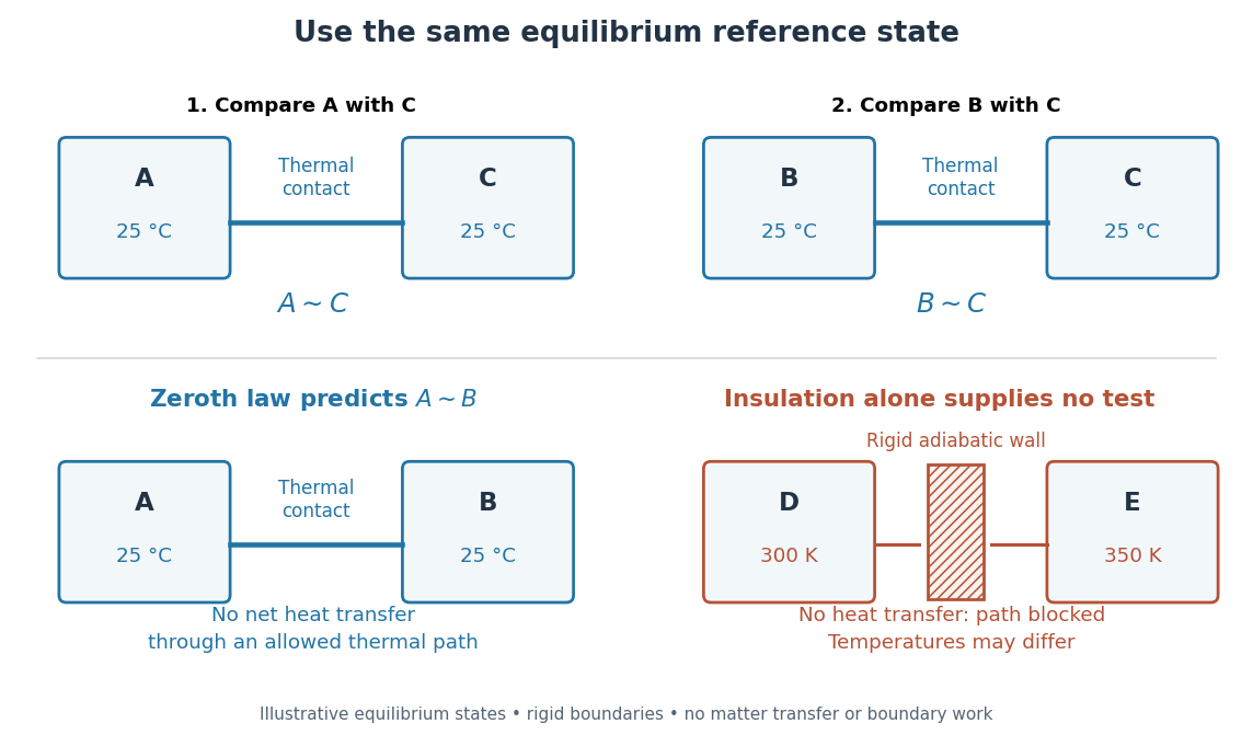
This explains why a thermometer can compare unlike materials: it supplies a reusable third system. A temperature is a property of an equilibrium state, while heat is energy transferred because of a temperature difference. Two bodies at the same temperature can have different internal energies and heat capacities. A thermometer therefore does not measure a body's stored amount of heat; the finite-body disturbance and waiting-time calculations in thermometer describe how making the comparison can change the state being measured.^[ref]

The name “zeroth” reflects logical order rather than the date of the first thermometer: this premise about thermal equilibrium precedes the already numbered first law of thermodynamics, Second law of thermodynamics and third law of thermodynamics. This is the naming explanation given in University Physics Volume 2 by Samuel J. Ling and others (§1.1, “Thermal Equilibrium”).^[ref]

The corresponding Zeroth law of black-hole mechanics states constancy of surface gravity over an equilibrium horizon; Hawking radiation identifies that quantity with physical temperature up to its universal conversion factor.

Put a contact thermometer $C$ in thermal contact with $A$, wait for thermal equilibrium, and record response $X_A$. Repeat with $B$ under the same operating constraints. If $X_A=X_B$, and the calibrated response is an injective function of temperature on this range, $C$ occupies the same thermal reference state in both comparisons. The zeroth law of thermodynamics then predicts $A\sim B$. Equality of raw numbers from different uncalibrated thermometers supplies no such premise.^[ref]

Use a probe whose participating heat capacity is small relative to each sample, or use maintained heat baths. Otherwise the matching readings describe the disturbed final states. Also hold the probe's immersion and mechanical conditions fixed: its response can depend on more than temperature. Matching readouts only tests agreement within resolution and repeatability, rather than proving exact equality of temperatures.

Agreement within a tolerance is not itself an equivalence relation. With a $0.10{}^{\circ }\mathrm{C}$ tolerance, readings $25.00$ and $25.16{}^{\circ }\mathrm{C}$ each agree with $25.08{}^{\circ }\mathrm{C}$, yet disagree with each other. This is a limitation of the measurement rule, not a failure of the exact transitivity asserted by the zeroth law of thermodynamics.