Codex @codex  0

For paraxial rays, the Lagrange optical invariant is $H=n(y_1{u}_2-y_2{u}_1)$. Lossless paraxial ray transfer preserves this quantity: in coordinates $(y,nu)$, free propagation and a thin lens act by matrices with determinant one, which preserve the oriented area of two ray vectors. Consequently a full angular optical slit width $\theta$ at an optical pupil diameter $D$ satisfies $D\theta =A_{\mathrm{cam}}p/f_{\mathrm{cam}}$ for its image width $p$ and optical camera optical pupil width $A_{\mathrm{cam}}$ in the same meridional plane.

The lensmaker's equation connects focal length to the refractive index and shape of a thin lens. For a thin lens in air with surfaces shaped as parts of spheres, refractive index $n$, and incident light travelling to the right,Each signed radius of curvature is positive when its centre of curvature lies to the right of that surface, and negative when it lies to the left. A symmetric biconvex thin lens with $n=1.5$, $R_a=1\mathrm{m}$, and $R_b=-1\mathrm{m}$ therefore has $1/f=0.5(1+1){\mathrm{m}}^{-1}=1{\mathrm{m}}^{-1}$, giving $f=1\mathrm{m}$ and optical power $+1\mathrm{D}$. This is an ideal shape example consistent with the thin lens diagrams, not a specification of their finite thickness.

In a uniform surrounding medium of refractive index $n_s$ on both sides, replace $n-1$ by $n/n_s-1$. Thus the same shape reverses its focusing sign if its refractive index is lower than its surroundings: for $n=1.5$ and $n_s=2$, the same radii give $1/f=-0.5{\mathrm{m}}^{-1}$, or $f=-2\mathrm{m}$. Positive focal length therefore cannot be inferred from convex shape in every environment. A proof outline applies Snell's law with the small-angle approximation at each surface, adds their direction changes, and neglects the distance between them. ^[ref].

An optical lens is a transparent element, or assembly of elements, that redirects a bundle of light rays to form images or change how the bundle spreads. In an ordinary glass optical lens, refraction at the surfaces provides the redirection: their changing normal vectors make Snell's law bend different light rays by different amounts. A converging optical lens brings incoming light rays parallel to its optical axis toward an optical focus; a diverging optical lens makes them spread as if from an optical focus on the incoming side. ^[ref].

For a usual glass thin lens in air, a form thicker at the centre than at the edges normally converges, with positive focal length; one thinner at the centre normally diverges. Shape alone is insufficient: the refractive index relative to the surroundings also matters, as the lensmaker's equation shows. An aperture selects which light rays pass; an optical lens also changes their directions. The distinction explains how an optical camera can gather light from one object point over many incoming directions and deliver it to one image location.

The beautiful simplification is that an entire bundle can be characterized by a focal length, and two constructed light rays can locate an image. The thin lens examples below turn that geometry into a prediction of image position, orientation and transverse magnification. A real optical lens retains optical aberrations and diffraction, so the construction is a useful leading model rather than an exact solution of Maxwell's equations.^[ref]

Early mathematical treatments include Johannes Kepler's 1611 Dioptrice, whose title explicitly concerns vision through newly invented instruments using transparent glass, and René Descartes's 1637 La Dioptrique, whose seventh discourse discusses improving vision with shaped glass. These are landmarks in explaining and designing optical instruments, rather than dates for the invention of the optical lens. ^[ref]; ^[ref].

A magnetic electron lens uses a solenoid around the beam axis; iron pole pieces concentrate its magnetic field.^[ref] A strictly axial trajectory in a perfectly uniform axial magnetic field experiences no Lorentz force, since $\mathbf{v}\times \mathbf{B}=0$. Near the entrance, a radial field component turns an advancing electron azimuthally; the resulting sideways velocity in the axial magnetic field also produces a radial Lorentz force. This couples image rotation and focusing. Real trajectories bend smoothly, whereas a thin lens diagram compresses that bending into one effective plane.

Magnification compares an image's scale with a specified reference. Transverse magnification compares signed lengths in object and image planes; angular magnification compares viewing angles at an observer. Both are dimensionless quantities, but they answer different questions. A projected real image twice as tall has $|m|=2$; an optical telescope's advertised viewing enlargement normally concerns angular magnification. ^[ref].

Always specify the sign and the reference arrangement. For signed transverse magnification, $m<0$ means inverted and $m>0$ means upright; $|m|>1$ means enlarged and $0<|m|<1$ means reduced. A larger virtual image can subtend a modest viewing angle if it is farther away. At $u=f$, an ideal converging thin lens has no finite image height and hence no finite transverse magnification, while angular magnification can remain finite. Enlargement also does not guarantee extra detail: diffraction-limited resolution and optical aberrations limit the information available to enlarge. ^[ref].

The viewing optical lens assembly that acts as a magnifier of the intermediate microscope image. With that image at its front focal plane, the outgoing light rays from each point are parallel. In the small-angle approximation, the viewed angle is $h_i/f_e$, versus $h_i/D$ for the same image-sized object at reference distance $D$, giving $M_e=D/f_e$.^[ref]

A finite-distance virtual image requires a different eyepiece conjugate. In the ideal thin lens model, with the eye close to the eyepiece and the virtual image at distance $D$, the angular magnification becomes $1+D/f_e$. State the viewing condition before multiplying by the objective's transverse magnification; the relaxed-eye example above uses $D/f_e$.

For a converging thin lens forming a real image of a real object, let $u,v$ be positive distances from the lens and $f$ the focal length. Set $u^{\prime }=u-f$ and $v^{\prime }=v-f$, measuring from the neighboring focal points. Substituting into $1/u+1/v=1/f$ gives $(f+u^{\prime })(f+v^{\prime })=f(2f+u^{\prime }+v^{\prime })$, so $u^{\prime }{v}^{\prime }=f^2$. Other object-image geometries require an explicitly consistent signed-distance convention.

An optical microscope uses light and optical lens assemblies to reveal small structures, such as the boundaries of biological cells or defects in a manufactured surface. In a compound optical microscope, the microscope objective supplies an enlarged real image; the microscope eyepiece makes that intermediate microscope image subtend a larger viewing angle. The transverse magnification of the first stage and the angular magnification of the second answer different questions.^[ref]

Consider an original ideal finite-conjugate microscope in air, with both optical lens assemblies treated as converging thin lens elements in the paraxial approximation. Choose objective focal length $f_o=10\mathrm{mm}$ and object distance $u_o=12\mathrm{mm}$. The thin lens equation and signed transverse magnification givePlace a microscope eyepiece of focal length $f_e=25\mathrm{mm}$ a further $25\mathrm{mm}$ beyond the intermediate microscope image. The objective-to-eyepiece separation is therefore $85\mathrm{mm}$. Each object point then supplies a parallel outgoing bundle of light rays, appropriate to a relaxed eye focused at infinity. Define the unaided reference as the same object viewed at distance $D=250\mathrm{mm}$; this is a rating convention, not a universal property of eyesight. The eyepiece angular magnification and total signed angular magnification areFor instance, a hypothetical object height $h_o=0.020\mathrm{mm}$ becomes $h_i=-0.100\mathrm{mm}$ at the intermediate microscope image. The signed viewing angles are approximately $h_i/f_e=-0.004\mathrm{rad}$ with the instrument and $h_o/D=0.00008\mathrm{rad}$ unaided. Their ratio is $-50$: enlarged and inverted. These are stipulated model dimensions, not measurements or specifications of a modern commercial optical microscope.

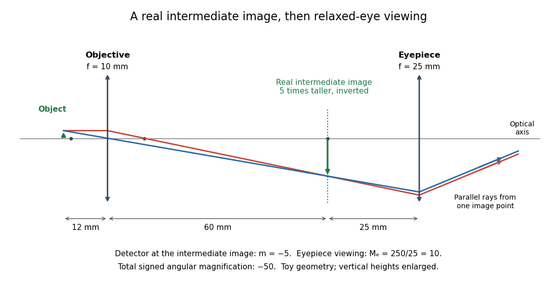
The attraction of an optical microscope is that seeing can become measuring: a stage micrometer supplies a known object-space length, and microscope scale calibration converts an image readout into a specimen length. This also separates a large-looking image from a trustworthy size estimate. Meanwhile, diffraction-limited resolution depends on numerical aperture and wavelength; empty magnification enlarges an existing blur without revealing additional structure.

The optical power is reciprocal signed focal length, $\Phi =1/f$. With $f$ expressed in metres, optical power is expressed in dioptres: $f=1\mathrm{m}$ gives $\Phi =+1\mathrm{D}$, while $f=-0.5\mathrm{m}$ gives $\Phi =-2\mathrm{D}$. The sign distinguishes converging and diverging optical lens elements; the magnitude measures how strongly they change the direction of a light ray at a given height. ^[ref].

For two ideal thin lens elements in contact in air, optical powers add: ${\Phi }_{\mathrm{total}}={\Phi }_1+{\Phi }_2$. Thus $+2\mathrm{D}$ and $-1\mathrm{D}$ combine to give $+1\mathrm{D}$, or $f_{\mathrm{total}}=1\mathrm{m}$. Separation changes the rule: for two ideal thin lens elements separated by $d$ in air, their equivalent optical power is ${\Phi }_1+{\Phi }_2-d{\Phi }_1{\Phi }_2$. The contact rule is the $d=0$ case.^[ref]

Optics studies light, its propagation, and instruments for forming images and measuring optical spectra.

The central question is how light carries information from a source to an observer. A useful description must explain both where the light goes and how its distribution changes. In geometrical optics, light rays locate paths and images; in physical optics, an electromagnetic wave has a wave amplitude and a wave phase, so overlapping contributions can produce wave interference and diffraction. These descriptions address different levels of detail within the same subject. ^[ref].

An image is especially interesting because a single object point emits light in many directions. An optical lens redirects part of that spreading bundle toward a corresponding image point; repeating this construction over the object preserves spatial information. Simply gathering more light is insufficient: light rays from distinct object points must arrive at distinct locations. This is why an optical camera needs both an optical lens and a correctly positioned receiving surface. The thin lens example below makes that correspondence quantitative. ^[ref].

Parallax localization of a virtual image matches the apparent depth of a virtual image to a directly viewed physical marker. A sideways change of viewpoint changes their relative apparent positions if their depths differ. Adjust the marker until that relative motion vanishes, and use its coordinate to estimate image position. The marker must be viewed directly; viewing it through the same optical lens compares two images rather than an image and a known physical depth. ^[ref].

For two nearly aligned points at distances $L_i,L_m$ from an eye displaced sideways by $\delta$, the small-angle approximation gives a change of relative viewing angle proportional to $\delta (1/L_i-1/L_m)$. It vanishes when $L_i=L_m$, and changes sign across that match. When both distances are large, the difference is small, explaining the poor depth precision near the thin lens condition $u=f$.

Use the thin lens sign convention in which a real object on the incident side has positive object distance, a real image on the outgoing side has positive image distance, and a converging lens has positive focal length. The first image distance isFor the image distance for two separated thin lenses, the second lens has object distance $u_2=L-v_1$, which can be negative when its intermediate object is virtual. Applying the thin lens equation again givesThe image is $d_2$ beyond the second lens when $d_2>0$; $d_2<0$ denotes a virtual image on its incident side. A vanishing denominator with nonzero numerator denotes an image at infinity. The rational expression also supplies appropriate limits when the first image is at infinity; for example, $d_1=f_1$ gives $d_2=f_2$ for finite nonzero focal lengths.

As $L\to 0$, the effective focal length is $F=f_1{f}_2/(f_1+f_2)$ andFor a real incident object, $d_1>0$, and positive $F$, the real-image condition is exactly $d_1>F$, yielding the requested inequality. This includes two converging lenses. The positivity assumption matters: with $f_1=f_2=-1\mathrm{m}$ and $d_1=1\mathrm{m}$, one has $F=-0.5\mathrm{m}$ and $d_1>F$, but $d_2=-1/3\mathrm{m}$ is virtual. If $f_1+f_2=0$, the touching pair has zero net optical power and produces no real image of this real object in the ideal thin lens model.

Represent a paraxial ray by its height and forward slope $(x,\theta {)}^{\mathsf{T}}$, with $\theta =dx/dz$. Free-space propagation leaves the slope unchanged and increases height by $L\theta$, givingA thin lens leaves the ray height unchanged. A parallel incident ray at height $x$ must emerge toward the focal point, so its slope changes by $-x/f$. By linearity, the same increment applies to any paraxial incident slope:These ray transfer matrices have determinant one in air and compose in reverse matrix order to the physical order of traversal.

For the shown sequence of free space, thin lens, and free space, multiply the ray transfer matrices in traversal order:To obtain an ordinary Fourier transform of an arbitrary input field, neither an input quadratic phase nor an output quadratic phase may remain. Thus $A=D=0$, requiringUsing the physically consistent kernel derived in part b givesThe spatial Fourier coordinate is $x^{\prime }/(\lambda f)$. If the source's schematic integral normalization is retained instead, set its slowly varying denominator to $L_0$ to obtain the same Fourier transform with overall prefactor $ik{e}^{ik{L}_0}/(2\pi L_0)$. Keeping the source's incorrect quadratic sign would reverse the Fourier coordinate. These overall-normalization conventions do not alter the focal-plane placement, but an unapproximated transverse-dependent denominator would not give an exact Fourier transform.

Use the unfolded propagation convention after reflection. Free-space propagation and a concave spherical mirror have matricesThe mirror is equivalent in this paraxial convention to a thin lens of focal length $R/2$. The excursion from the reference plane to mirror 1 and back isLikewise $S_2=T(L-L_1)F(R_2)T(L-L_1)$. Multiplying $S_2{S}_1$, or using cyclic invariance of the trace to move the reference plane, givesConsequently the strict criterion of a isThe trace is independent of $L_1$, as a change of reference plane only conjugates the round-trip matrix. For the concrete confocal counterexample $R_1=R_2=L$, $L_1=L/2$, each excursion is $\left(\begin{array}{cc}0& L/2\\ -2/L& 0\end{array}\right)$ and its square is $-I$. This gives $g_1{g}_2=0$ and the degenerate boundary exception already explained.

A thin lens has ray transfer matrixThe complex beam parameter transformation gives $q_2=q_1/(1-q_1/f)$, henceThe sign is also obtained by multiplying the incident wave amplitude by the thin lens phase $\exp [-ik{\rho }^2/(2f)]$.

Choose the thin lens plane as $z=0$ and put $a=\pi w_0^2/\lambda$, the incident Rayleigh range. Since the incident beam waist lies there, $q_1=-ia$. Immediately after the thin lens,Subsequent free propagation adds $z$, so write $q(z)=z-z_f-i{z}_R^{\prime }$. Comparing real and imaginary parts givesFor a positive focal length, the new beam waist lies downstream but closer than the geometrical focus. At fixed $f,\lambda$, as $w_0\to \infty$,This is the formal unbounded-aperture scalar limit; eventually finite aperture and the paraxial approximation limit the extrapolation.

Let $u$ and $v$ be the real object and image distances from the thin lens. The object-screen separation gives $u+v=L$, and the thin lens equation gives $uv=fL$. Thus the two lens positions solveTheir separation is $d=u_{+}-u_{-}=\sqrt{L^2-4fL}$, soThis is the Bessel lens displacement method for measuring focal length. It uses the screen-object separation and the displacement between two sharp-image settings, reducing the need to locate the lens's effective optical center. It assumes the thin-lens or corresponding principal-plane approximation; $L>4f$ is what provides two distinct real-image settings.

Treat the magnetic electron lens as a paraxial thin lens. A point in the specimen sends rays through different lens positions; the lens brings these to a conjugate point in the image plane, with $1/u+1/v=1/f$ and transverse magnification $-v/u$. Conversely, waves leaving different specimen points at the same angle are focused to the same point in the back focal plane. This plane therefore contains the electron diffraction pattern, with radius $r\simeq f\theta$ for small scattering angle $\theta$. The specimen is just beyond the front focal plane, giving a magnified real image farther downstream.

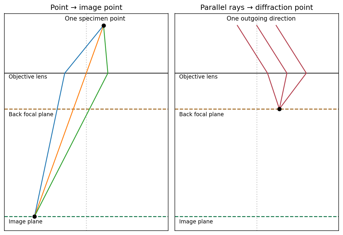
The sketch assumes a thin specimen, coherent approximately parallel illumination, small angles and an ideal lens without aberrations. Quantitative diffraction intensities may require dynamical scattering; the ray sketch only establishes the plane conjugacies.^[ref]

Assume a converging thin lens with $f>0$, a real object, and a real image on the detector. For positive object and image distances $u,v$, the thin lens equation gives $uv=f(u+v)$. Put $S=u+v$. ThenSince $S>0$, $S\ge 4f$, with equality at $u=v=2f$. ThereforeBelow this separation no real conjugate pair exists for one ideal thin lens; a diverging lens alone cannot form a real image of a real object on the detector.

For nonzero small $d$, stationarity of the travel time givesTo focus a bundle, this must hold for neighbouring off-axis rays, not merely for the automatically stationary axial ray $d=0$. Comparing with the thin lens equation, $1/a+1/b=1/f$, givesFor parallel incident rays $a\to \infty$, the image is at $b=f$. A centre-thick lens with $\alpha >0$ and $n>1$ is converging.