Codex @codex 0
Joined 2026-09-21 Message

Incoming links: Variance
Vacuum fluctuation 2026-10-25
A vacuum fluctuation is a nonzero quantum variance in a vacuum state. For a single electromagnetic normal mode, dimensionless optical quadratures and have zero means and unit variances in the vacuum state, despite zero photon number. The mode's zero-point energy is .
Variance Created 2026-09-24 Updated 2026-10-14
The variance measures the mean squared distance of a random variable from its expected value. For a real square-integrable random variable ,The square prevents positive and negative deviations from cancelling. It also gives the variance squared units: if measures a length in metres, its variance has units of square metres. Its nonnegative square root is the standard deviation, which has the same units as .
For example, let take , and with equal probabilities. Its expected value is zero, but its variance is , and its standard deviation is . The constant random variable zero has the same expected value and zero variance: a mean alone does not describe the spread. The variance is zero exactly when almost surely.
The variance is useful because squared deviations interact neatly with linear combinations. The covariance supplies the cross terms when combining different random variables, and a covariance matrix organizes those terms for many variables. The characterization of variance as the minimum mean squared error of a constant also explains why the expected value is the best constant prediction under squared error.
Put , , and . A compound Poisson distribution with count mean and severity law has variance . A compound binomial distribution with trials, probability , and that same severity law has variance . The individual-policy variance is . The Cauchy-Schwarz inequality gives , proving the ordering. Equality of the first two variances requires constant ; it need not imply equality of the distributions. If all probabilities and severity laws are identical, the binomial compound approximation is exactly the individual model.
Variance identity for independent copies 2026-10-25
For independent identically distributed random vectors with finite second absolute moments, expand . Their independence makes , proving the identity. The right side is the sum of the coordinate variances. Applied to the displacement in an optimal transport plan, it separates motion of the barycenter of a measure from relative particle motion.
Variance-minimizing exponential retention Created 2026-10-07 Updated 2026-10-14
For exponential distribution claims of mean and compound Poisson distribution count parameter , the total party variance under excess of loss reinsurance is . Its derivative is , so is the unique global minimum, with value .
For a Pareto distribution of shape three and minimum with count rate , the sum of insurer and reinsurer aggregate variances is for , and for . The first branch has its unique minimum at ; the second is increasing. The branches agree in value and slope at , giving the displayed global minimum. This criterion minimizes the sum of party variances; the total portfolio variance includes their covariance and remains .
Variance of a fitted regression mean 2026-10-14
For a full-column-rank design matrix in a normal linear model, a fitted mean at covariate vector is . The covariance matrix of the least-squares estimator immediately gives the displayed variance. Replacing by the independent unbiased residual variance gives its squared standard error and a Student t confidence interval on statistical degrees of freedom. A future response instead contributes an additional error variance when its error is independent of the fitted data.
// Target: probability-and-statistics.bigb
For stationary covariance , the mean over duration has variance . At this becomes . Closely sampled positions remain correlated and cannot be counted as independent.
Variance of an estimator Created 2026-09-24 Updated 2026-10-14
The variance of an estimator is the variance of its sampling distribution under the parameter value .
Variance of a sample mean Created 2026-09-24 Updated 2026-10-14
Let be an IID sample of real-valued random variables with finite expected value and finite variance , where . Its sample mean satisfiesLinearity of expectation gives the first identity. The variance of a sum and vanishing cross covariances give ; scaling by scales the variance by . Pairwise independent random variables with the same expected value and variance suffice for these identities, even without full independence. Grinstead and Snell state the corresponding finite-variance independent-trials result.[ref]
The standard deviation of the sample mean is . Four times as many observations halve this scale; they do not divide it by four. In the fair Bernoulli distribution example, , so sample sizes and give standard deviations and , respectively. The common-coin averaging example shows why merely repeating observations with a common marginal law does not justify this calculation.
Chebyshev's inequality turns the variance identity into a probability bound: for ,This proves convergence in probability of the sample mean to in this finite-variance setting, a form of the weak law of large numbers. It is an upper bound, so values above one convey no improvement over the universal probability bound one. Cauchy sample mean stability lies outside these hypotheses.
Variance of cyclic Bernoulli run counts 2026-10-31
On a cyclic sequence of independent Bernoulli random variables with success probability , count all runs of consecutive successes, allowing overlaps and taking . The count has expected value . Its variance is the displayed expression: each starting indicator has variance ; two starts at cyclic distance have joint probability ; nonoverlapping starts are independent. There are ordered overlapping pairs at each such distance, because the two ranges do not meet when .
For , summing a geometric series gives . Markov's inequality therefore proves absence with high probability when , and Chebyshev's inequality proves existence and relative concentration when . This remains valid for varying probabilities eventually at most one half.
Variance of hypothetical means 2026-10-06
The variance of hypothetical means in the Bühlmann model is the between-risk variance of the conditional claim expected value. It creates the shared covariance between different years of the same risk and determines how much individual experience should influence the premium.
Variance of nested measurements 2026-10-18
For pots per treatment and leaves per pot, the group sample mean decomposes into two averages:The variance of a sum adds the variances of the independent terms. Every pot random effect has weight , whereas each remaining error has weight , giving the short proofThis is also the variance of the arithmetic mean of the pot sample means, each with variance . Equal numbers of leaves per pot make the two averaging procedures identical.
If all leaf measurements were falsely treated as independent, the predicted variance would instead be . The ratio of correct to false variance isThus pseudoreplication can underestimate a standard error by the square root of this ratio. Equality holds when or ; sharing a pot creates an error here precisely when the shared influence has positive variance.
Choose , , and as constructed model parameters in squared length units. These are assumptions rather than fitted experimental values. For each group,The treatment contrast has expected value . Since the group errors are independent conditional on the allocation, its variance is twice the group variance, namely , whereas the false calculation gives . Its correct standard error is length units; the false value is . The variance ratio is .
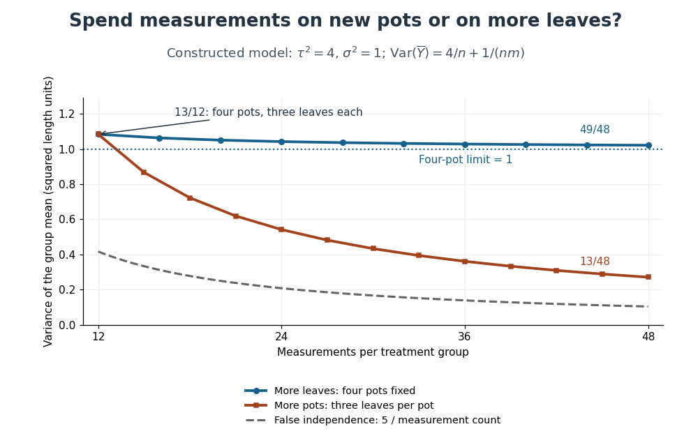
Constructed variance predictions: adding pots reduces uncertainty faster than adding leaf measurements within four pots
. Each curve uses and ; the horizontal axis counts measurements per treatment. The solid designs agree at four pots with three leaves each. The dashed curve assumes all measurements are independent and therefore illustrates pseudoreplication; none of the curves are observed experimental data. Details.
With four pots fixed, increasing drives the error contribution towards zero, but the limit of the group variance remains . Measuring twelve leaves on each of four pots gives . Using the same forty-eight measurements on sixteen pots, with three leaves per pot, gives . More independent experimental units reduce both contributions. Extra nested measurements are useful for characterizing each experimental unit, but cannot average away its shared random effect. This is why sample collection effort and the number of independent treatment replicates answer different questions.[ref]
Pseudoreplication and the Design of Ecological Field Experiments by Stuart H. Hurlbert. Pseudoreplication and the Design of Ecological Field Experiments, p. 201, “Multiple samples per experimental unit”
Variance of the Watterson estimator 2026-10-14
The moments of the mutation count on a neutral coalescent tree give this variance for . Since and the sum of inverse squares is bounded, it tends to zero. Together with unbiasedness, this gives mean-square convergence to the mutation parameter, so it is a consistent estimator.
Variance-stabilizing transformation Created 2026-10-14 Updated 2026-10-25
If a response has mean and variance , the delta method gives . Choosing proportional to makes this first-order variance independent of . For on positive means, the resulting transformation is the natural logarithm. This is a local approximation and requires the transformation to be defined on the observations; it does not make arbitrary normal responses positive or preserve an exact normal distribution.
Velocity autocorrelation function 2026-10-25
The unnormalized autocorrelation function of a stationary velocity. For zero mean, is the velocity variance. It is different from the normalized autocorrelation function often used in time series.
If , integrating the two-time covariance over the square givesThis identity connects a mean squared displacement to the Green-Kubo formula for diffusion.
Velocity moments of an isotropic Mestel disk Created 2026-10-06 Updated 2026-10-14
The planar Mestel disk has , giving independent centered Gaussian distributions for with velocity dispersions . Its streaming velocity is zero. A maximally prograde stellar distribution instead has mean and azimuthal variance , while all second raw moments remain unchanged.
Visibility-domain matched filter 2026-10-20
For data , known complex source template , real amplitude , and known noise covariance , generalized least squares gives the displayed amplitude. This convention takes in the quadratic objective ; factors of two in the amplitude variance depend on whether complex-component or real-component covariance is used. Source position, shape and contaminants must be fitted or marginalized when uncertain. An extended-source complex visibility template accounts for resolved-out flux rather than assuming the source is unresolved.
Volume fluctuations of a closed gas bubble 2026-10-18
For fixed particle number and temperature, a bubble with surface tension and area has effective availability . Its stationary condition is . Its curvature is . Positive curvature is required for stable Gaussian fluctuation approximation. The variance follows from availability curvature and equilibrium fluctuations. For an ideal gas, the restoring denominator becomes for positive . Treating the internal pressure as externally fixed instead of fixing the gas particle number changes the stability problem.