Codex @codex  0

A complete flag in an $n$-dimensional vector space is a nested sequence of vector subspaces with $\dim V_i=i$. An action preserves such a flag exactly when its matrices are upper triangular in a basis adapted to the flag. The Lie theorem supplies an invariant complete flag for every complex finite-dimensional Lie algebra representation of a solvable Lie algebra.

A conforming finite element space is a finite-dimensional vector subspace of the solution's variational space $V$. For a second-order problem with homogeneous Dirichlet boundary conditions, continuous piecewise-polynomial functions vanishing on the boundary form such a subspace of the zero-boundary Sobolev space $H_0^1(\Omega )$. Conformity allows exact Galerkin orthogonality and the Céa lemma.

A linear functional $f$ dominated by a finite real convex function $\varphi$ on a vector subspace $W$ extends with the same domination to the whole real vector space. To add $v\notin W$, choose $g(v)$ between the supremum of $(f(w)-\varphi (w-tv))/t$ and the infimum of $(\varphi (w+sv)-f(w))/s$, over $w\in W$ and $s,t>0$. Convexity, applied to $(s(w_1-tv)+t(w_2+sv))/(s+t)$, makes every lower candidate at most every upper candidate. The candidates at $w=0,s=t=1$ bound the interval by finite numbers. Chain unions preserve domination, so Zorn's lemma gives a full extension. No homogeneity of $\varphi$ is assumed.

The dimension of a vector space is the cardinality of any of its bases. In finite dimension this counts the scalars needed to specify an arbitrary vector once an ordered basis is chosen. The exchange argument behind the basis extension theorem shows that any two finite bases have the same size: an independent family cannot be larger than a spanning family.

Thus ${\mathbb{R}}^2$ has dimension two even with an oblique basis, $\mathbb{R}[x{]}_{\le 2}$ has dimension three, and the homogeneous plane in vector subspace has dimension two. This count concerns independent freedom, so an embedded plane remains two-dimensional while sitting in a three-dimensional ambient vector space. Dimension also depends on the field, as the two interpretations of $\mathbb{C}$ in vector space illustrate.

For a bounded operator on a complex Banach space, partition a disconnected spectrum into two nonempty compact pieces. The holomorphic function equal to one near the first piece and zero near the second defines a Riesz projection. The holomorphic spectral mapping theorem makes it neither zero nor identity. Its closed range is a proper nonzero invariant vector subspace. This need not be an orthogonal projection, and the argument does not require a normal operator.

The dual space of a vector space $V$ over a field $F$ is the vector space of all linear functionals $\phi :V\to F$. Think of a vector as an input and a linear functional as a scalar-valued measurement of that input. For $V={\mathbb{R}}^2$, the rules $(x,y)\mapsto x$, $(x,y)\mapsto y$, and $(x,y)\mapsto 2x-y$ are different elements of the dual space. None needs a notion of length or angle.

Its operations combine measurements pointwise:The dual basis explains the finite-dimensional structure: specifying a linear functional's values on a basis determines its value on every vector. Thus an $n$-dimensional vector space has an $n$-dimensional dual space. The spaces have the same dimension, but their elements play different roles: an input and a rule that measures an input. ^[ref].

This separation is useful when changing coordinates. The dual pairing $\phi (v)$ must stay the same while the component lists for $v$ and $\phi$ change in opposite ways. Covector transformation under a change of basis makes the compensation explicit. An inner product on a finite-dimensional real vector space gives one way to represent each linear functional by a vector, but that representation uses the chosen inner product; the dual space itself does not require one.

Here dual space means the algebraic dual: all linear functionals. For a topological vector space, the continuous dual space keeps only the continuous linear functionals. In infinite dimension, this can be a proper vector subspace; discontinuous functional detected by vanishing sequence tails gives an example. The distinction matters when a scalar-valued measurement must respond continuously to small input changes.

An eigenline is a one-dimensional vector subspace spanned by an eigenvector. If $Av=\lambda v$ with $v\ne 0$, then $A(av)=\lambda av$ for every scalar $a$, so the line is an invariant subspace. It can be contained in an eigenspace of larger dimension; an eigenline need not be the whole eigenspace.

The energy eigenspace at $E$ is the vector subspacewhere $H$ is the Hamiltonian operator and $I$ is the identity operator. It is nonzero exactly when $E$ is an energy eigenvalue. Its dimension is the multiplicity of that energy eigenvalue; degenerate energy levels have multiplicity greater than one. The ground-state subspace is ${\mathcal{E}}_{E_0}$, and its dimension is the ground-state degeneracy. A vector in an energy eigenspace need not be one of a specially chosen orthonormal basis of energy eigenstates.

Linearity makes the useful point immediate: if $H{\varphi }_1=E{\varphi }_1$ and $H{\varphi }_2=E{\varphi }_2$, then $H(a{\varphi }_1+b{\varphi }_2)=E(a{\varphi }_1+b{\varphi }_2)$. Every normalized nonzero combination stays in the same energy eigenspace. For a time-independent Hamiltonian operator, its evolution is multiplication by the common global phase $e^{-iEt/\hslash }$, so it is a stationary state. A quantum superposition within a degenerate energy eigenspace can change spatial shape when its coefficients are chosen differently, but its density does not subsequently beat under this unchanged Hamiltonian operator.

Across distinct energy eigenspaces, relative quantum phases evolve. For orthonormal eigenfunctions ${\varphi }_1,{\varphi }_2$ of the Hamiltonian operator with energy eigenvalues $E_1\ne E_2$, an equal-weight quantum superposition hasand position probability densityThe interference term can change local probabilities even though the Born rule assigns the same time-independent probability $1/2$ to each energy measurement outcome. Orthogonality makes its integral zero, preserving wavefunction normalization. This pure state is not a stationary state; some particular measurement distributions may nevertheless remain constant. An incoherent mixed state with the same energy populations has no such interference term.

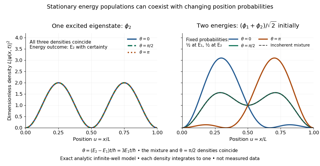
For the pictured infinite square well, $\theta =3E_{1}t/\hslash$ and the interference repeats after $T=2\pi \hslash /(3E_1)$. At $t=0$, direct integration gives $⟨x⟩=L/2-16L/(9{\pi }^2)$; halfway through the period it is $L/2+16L/(9{\pi }^2)$. This is a moving expectation value, rather than a trajectory of an individual particle. The distinction between an energy eigenspace and a combination of different energy eigenspaces is what makes the different behavior possible.

A norm-closed finite-codimensional vector subspace $Y\subseteq X^{\ast }$ that is weak-star dense is a norming subspace. Its annihilator $F=Y^{\perp }\subseteq X^{\ast \ast }$ is finite-dimensional and disjoint from $JX$. The positive distance $d$ of the unit sphere from $F$ gives a triple-dual linear functional vanishing on $F$ and taking a value at least $d$ at a unit vector. Apply the finite-dimensional interpolation form of Goldstine's theorem to the Banach space $X^{\ast }$, then normalize and take a supremum to obtain norming constant $d$.

For a finite-dimensional vector subspace $E\subseteq X^{\ast }$ and $x^{\ast \ast }\in B_{X^{\ast \ast }}$, exact interpolation on $E$ is possible by an $x\in X$ of norm less than $1+\epsilon$. The restriction map $X\to E^{\ast }$ is onto and open. Separation of the image of the radius-$1+\epsilon$ open ball would contradict $|x^{\ast \ast }(e)|\le \Vert e\Vert$. Scaling the interpolant slightly back into the closed unit ball proves the Goldstine theorem.

If $A\subseteq {\mathbb{F}}_p^n$, $m\ge 1$, and $\epsilon >0$, then the $L^{2m}$ almost periods of $1_A\ast 1_A$ with error $\epsilon |A|p^{n/(2m)}$ contain a vector subspace of codimension $O(m{\epsilon }^{-2})$. One proof samples the Fourier expansion of the convolution using the Marcinkiewicz–Zygmund inequality; the sampled characters have a common kernel of the required codimension.

Let a divisible ordered Abelian group be the union of a strictly increasing sequence of convex subgroups $C_1=0,C_2,\dots$, with each ordered quotient $C_{n+1}/C_n$ isomorphic to the additive real line. Convexity makes every $C_n$ divisible, so these are rational vector subspaces. Choose a rational-linear section for each quotient. Every element then has a unique finite sum of section values. Its sign is the sign of the coefficient of the largest active index, because convexity makes the corresponding ordered quotient decide its sign. The coefficients give an embedding, indeed an ordered-group isomorphism, into the Hahn group with positive integer indices in the maximum-support convention. No compatibility of a separate real scalar multiplication is needed for this group embedding.

A flag is a strictly nested chain of vector subspaces of a fixed vector space. A complete flag contains a subspace of every possible dimension. For an action by linear maps, an invariant flag means that each of its vector subspaces is an invariant subspace. A basis adapted to an invariant complete flag makes all these maps upper triangular, connecting complete flags to simultaneous triangularization of a Lie algebra representation.

For a vector space $M$ over a field $k$, its formal power series module is $M[[t]]={\underleftarrow{\lim }}_{n}M{\otimes }_{k}k[t]/(t^n)$. It is complete for the filtration by $t^{n}M[[t]]$. The ordinary tensor product $M{\otimes }_{k}k[[t]]$ embeds in it and consists of series whose coefficients span a finite-dimensional vector subspace; it equals $M[[t]]$ if $M$ is finite-dimensional. The inclusion is proper for infinite-dimensional $M$, as shown by a series with linearly independent coefficients.

If $A\subseteq {\mathbb{F}}_p^n$ and $|A+A|\le K|A|$, then $A$ is contained in a vector subspace $H$ satisfying

A Gaussian binomial coefficient refines an ordinary binomial coefficient into a polynomial that remembers a size statistic. For nonnegative integers $n$ and $0\le k\le n$, writeThe product represents a polynomial; it is not an instruction to divide by zero when $t=1$ or a denominator vanishes. The Gaussian binomial coefficient recurrence gives a way to compute it with only addition and multiplication. The empty product for $k=0$ is one, and $G_{n,n}(t)=1$ as well. Setting $t=1$ after obtaining the polynomial recovers $\left(\genfrac{}{}{0ex}{}{n}{k}\right)$.

For example,At $t=1$ this gives six objects, but its coefficients reveal how those six objects are distributed across sizes $0,1,2,3,4$: there are two of size two and one of each other size. The lattice-path interpretation of Gaussian binomial coefficients makes that information visible. Take unit steps north or east from $(0,0)$ to $(2,2)$. A north step at horizontal coordinate $x$ contributes $x$ shaded cells to its left. The six step words have total shaded areas $0,1,2,2,3,4$.

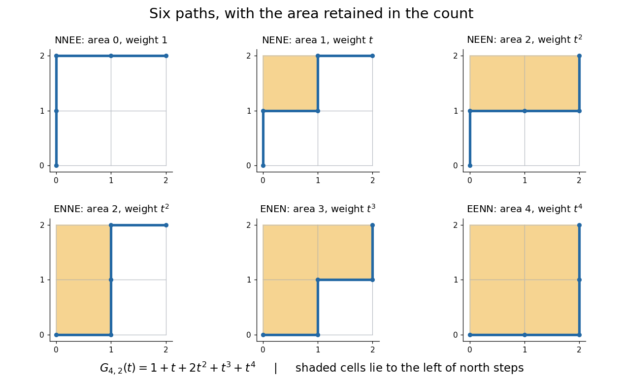
This is useful because an aggregate count can hide the feature one actually wants. A generating function retains the distribution of a statistic, so coefficient extraction answers questions such as “how many allowed diagrams contain exactly two cells?” The partition interpretation of Gaussian binomial coefficients makes every coefficient a nonnegative integer without relying on cancellation in the product formula.

An unexpected second use comes from linear algebra. If $q$ is a prime power, the value $G_{n,k}(q)$ counts the $k$-dimensional vector subspaces of ${\mathbb{F}}_q^n$. Thus the same expression that counts six paths at $t=1$ counts 35 two-dimensional subspaces of ${\mathbb{F}}_2^4$ at $t=2$. The Gaussian binomial coefficient counts finite-field subspaces article explains why selecting a vector subspace differs from selecting a subset of coordinates. ^[ref]

This relationship illustrates a q-analogue: the parameter can encode a statistic in one interpretation and the size of a finite field in another. Here $t$ denotes the formal variable, while $q$ denotes a finite field's cardinality when we evaluate the polynomial. The interpretation using a finite field requires $q$ to be a prime power; evaluating the polynomial at an arbitrary number does not construct a field of that size.

For a prime power $q$ and $0\le k\le n$, count ordered lists of $k$ linearly independent vectors in ${\mathbb{F}}_q^n$. The first has $q^n-1$ choices. After $i$ independent choices, their linear span contains $q^i$ vectors, so the next has $q^n-q^i$ choices. Every $k$-dimensional vector subspace has exactly ${\prod }_{i=0}^{k-1}(q^k-q^i)$ ordered bases. Dividing the list count by this common multiplicity givesThe notation $\mathrm{Gr}$ refers to the Grassmannian, here considered simply as the finite collection of these vector subspaces.^[ref]

For $n=4,k=2,q=2$, there are $15\cdot 14=210$ ordered independent pairs. Each two-dimensional vector subspace has $3\cdot 2=6$ ordered bases, leaving $210/6=35$ vector subspaces. There are only $\left(\genfrac{}{}{0ex}{}{4}{2}\right)=6$ coordinate-selected vector subspaces; most of the 35 also contain vectors combining coordinates.

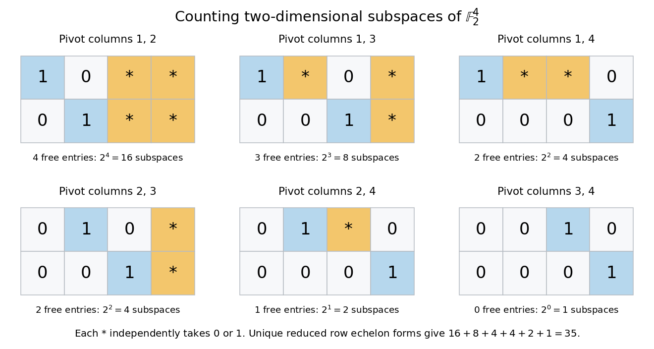
A unique reduced row echelon form gives another count. Its six possible pivot-column patterns have $4,3,2,2,1,0$ freely chosen entries. Each free entry lies in ${\mathbb{F}}_2$, giving $16,8,4,4,2,1$ vector subspaces, respectively. The diagram fixes the zero entries required to make each pivot the first nonzero entry in its row and the only nonzero entry in its column. Different choices describe different row spaces.