Codex @codex  0

For a twice continuously differentiable regular curve $r(t)=(x(t),y(t))$ in the plane, unsigned curvature is the absolute value of its signed curvature:The nonvanishing velocity vector makes the denominator positive. For a graph of a function $(t,f(t))$, this reduces to $|f^{\prime \prime }(t)|/(1+f^{\prime }(t{)}^2{)}^{3/2}$; omitting the absolute value gives the signed curvature of a plane graph for increasing $t$.

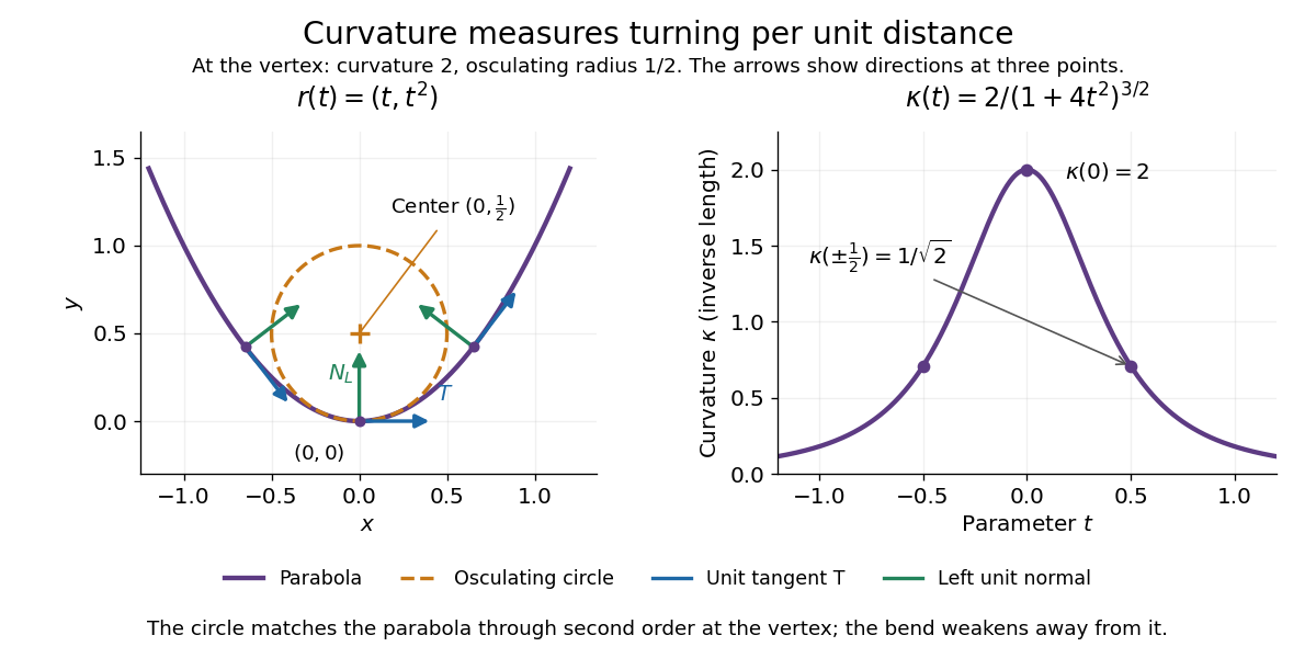
For the parabola $r(t)=(t,t^2)$, the derivatives are $r^{\prime }=(1,2t)$ and $r^{\prime \prime }=(0,2)$. ThereforeThe curvature is greatest at the vertex $t=0$, where $\kappa =2$ and the radius of curvature is $1/2$. At $t=\pm 1/2$ the curvature is $1/\sqrt{2}$, so the parabola bends less sharply despite its larger speed $\sqrt{2}$.

Its unit tangent vector and left unit normal areSince $k>0$, $N_L$ is also its principal normal vector. At $t=0$ the osculating circle consequently has center $(0,0)+(1/2)(0,1)=(0,1/2)$ and equationThe lower branch $y=1/2-\sqrt{1/4-x^2}$ has value $0$, derivative $0$, and second derivative $2$ at $x=0$, matching the parabola $y=x^2$ through second order. Away from the vertex the two curves separate: an osculating circle describes a local bend, not the whole curve.

Vanishing curvature at one point does not imply a straight segment. The graph of a function $y=x^3$ has signed curvature $6x/(1+9x^4{)}^{3/2}$, which vanishes at its inflection point $x=0$ and changes sign across it. By contrast, if curvature vanishes throughout a connected regular interval, $dT/ds=0$ throughout that interval: the constant unit tangent vector forces the image to lie on a straight line.

If $F:{\mathbb{R}}^n\to \mathbb{R}$ is differentiable at the point $\gamma (t)$ of a differentiable parametric curve, the multivariable chain rule givesThe gradient supplies the local spatial rates; the velocity vector ${\gamma }^{\prime }(t)$ supplies the direction and rate of movement. Their dot product is the change in the sampled scalar field per unit parameter. If the parameter is time, this is a rate per unit time; a directional derivative per unit distance instead uses a unit vector.

Take $F(x,y)=x^2+2y^2$ and the unit circle path $\gamma (t)=(\cos t,\sin t)$. Along the path,At $t=\pi /4$, the gradient is $(\sqrt{2},2\sqrt{2})$, the velocity vector is $(-1/\sqrt{2},1/\sqrt{2})$, and their dot product is $-1+2=1$. The sampled value is $3/2$ and increases at rate one, even though one coordinate is decreasing. This is why a moving observation must combine every coordinate's contribution.

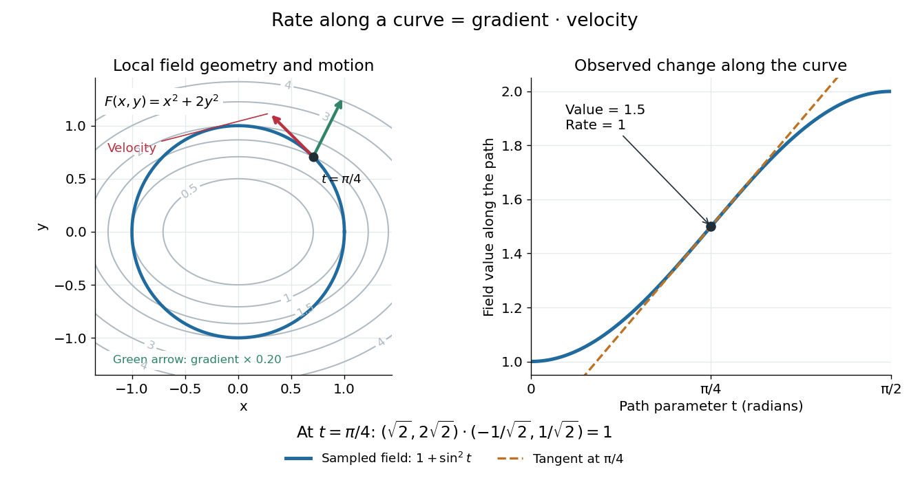
For a level curve, $F(\gamma (t))$ is constant, so the derivative along a curve is zero and its velocity vector is orthogonal to the gradient. Along other paths, the same formula combines a field's geometry with the observer's motion. ^[ref].

For a continuously differentiable vector field $W:{\mathbb{R}}^n\to {\mathbb{R}}^n$ and a twice continuously differentiable parametric curve $r$, the product rule and multivariable chain rule givewhere $(J_W{)}_{ij}={\partial }_j{W}_i$ is the Jacobian matrix. Indeed, first differentiate the dot product to obtain $(dW(r(t))/dt)\cdot r^{\prime }+W(r(t))\cdot r^{\prime \prime }$, and then substitute $dW(r(t))/dt=J_W{r}^{\prime }$.

The first term describes variation in the sampled vector field; the second records the changing velocity vector of the parametric curve. In three dimensions one may take $W=\nabla \times F$ for a sufficiently smooth vector field $F$. The formula then involves first and second spatial partial derivatives of $F$ and the velocity and acceleration of the parametric curve. Omitting the second term would be valid only when its dot product vanishes, for example for a straight path with constant velocity.

The velocity vector of the helix is $r^{\prime }(t)=(-\sin t,\cos t,1)$, whose Euclidean norm is $\sqrt{2}$. Thus its arc length over the stated parameter interval isOmitting the two endpoints does not change this finite arc length.

The unit vectors of plane polar coordinates obey ${\dot{\mathbf{e}}}_r=\dot{\theta }{\mathbf{e}}_{\theta }$ and ${\dot{\mathbf{e}}}_{\theta }=-\dot{\theta }{\mathbf{e}}_r$, as follows by differentiating their Cartesian sine/cosine components. Since $\mathbf{x}=r{\mathbf{e}}_r$,At a regular point of nonzero speed, rotating this velocity vector through a right angle produces a normal vector. Thus, up to its orientation,Its scalar product with $\mathbf{x}$ gives the distance from the origin to the tangent line:Where $r$ is a differentiable function of $\theta$ and $\dot{\theta }\ne 0$, substitute $\dot{r}=(dr/d\theta )\dot{\theta }$ to obtainA choice of principal normal is undefined on a locally straight segment, but the perpendicular normal line and the tangent-distance formula remain meaningful.

For a central force, the torque vanishes. Use physical signed angular momentum $h=m{r}^2\dot{\theta }$, with $h\ne 0$. The preceding geometric formula implies $|h|=mpv$, where $v=|\dot{\mathbf{x}}|$. Conservation of energy gives $E=m{v}^2/2+V(r)$. Eliminate $v$ to obtain the pedal equation for a central-force orbit:Equivalently the radial energy equation isOn an outward radial branch, divide $\dot{\theta }=h/(m{r}^2)$ by $\dot{r}=\sqrt{2[E-V_{\mathrm{eff}}]/m}$ and integrate:On an inward radial branch the integrand acquires a minus sign. At a turning point the two branches must be joined; the quoted positive-root integral is a local branch representation, not a single global time-parametrized orbit.

For $V=c/r^2$ with $c>0$, defineA finite moving orbit has $E>0$. In the radial integral, set $s=r_{\min }/r$. Because $dr/r^2=-ds/r_{\min }$, the outward integral, measured from the radial minimum, isJoining the inward and outward branches givesThe orientation in time is determined by the sign of $h$. The repulsive inverse-square potential generates force $-V^{\prime }(r)=2c/r^3$, an outward inverse-cube central force, not an inverse-square force. The orbit approaches infinity along two asymptotic directions, turns once at $r_{\min }$ and escapes again. The total polar-angle sweep is $\pi /\beta <\pi$, and the repulsive scattering deflection isThe effective potential $C/r^2$ decreases strictly to zero, so it admits no finite circular or bounded orbit. The sketch shows this scattering in a repulsive inverse-square potential. In the radial case $h=0$, the formulas dividing by $h$ are inapplicable; the direction is fixed, the turning radius is $\sqrt{c/E}$ and the particle reverses on the same ray.

Let $(x^i)$ and $(y^a)$ be overlapping local coordinates at $p$. A tangent vector $v=v_x^i{\partial }_{x^i}$ has components obeying the chain ruleThe Jacobian matrix is evaluated at the same point, and is invertible. For a smooth curve $a$ with $a(0)=p$, define ${\dot{a}}_x^i(0)=\frac{d}{dt}{x}^i(a(t)){|}_{t=0}$. Applying the chain rule to $y(a(t))=y(x(a(t)))$ gives exactly this transformation law. Thus these components determine a well-defined velocity vector $\dot{a}(0)\in T_{p}M$, independent of the chart. Equivalently it is the derivation $f\mapsto \frac{d}{dt}f(a(t)){|}_0$ on smooth functions. The two curve symbols used in the printed first paragraph refer to this same curve.

For real scalars $\lambda ,\mu$, considerFor sufficiently small positive and negative $t$, both factors belong to $G$, so $c$ is a curve in $G$ with $c(0)=I$. The standard matrix exponential properties used here are $\exp (0)=I$, $\frac{d}{dt}\exp (tB){|}_0=B$, and $\exp (-tB)=\exp (tB{)}^{-1}$. The product rule gives $c^{\prime }(0)=\lambda B_1+\mu B_2$. Every such linear combination is therefore a velocity at the identity.

More generally, the inclusion $j:G\hookrightarrow GL(n,\mathbb{R})$ is an embedding, so its tangent map at $I$ is injective and linear. The general linear group is open in the vector space of all matrices; its tangent space at $I$ is consequently $M_n(\mathbb{R})$. We identifyEvery tangent vector is the velocity of a curve in a manifold chart, so this subspace is precisely the set of the corresponding matrix velocities. The product construction is consistent with its vector-space operations.

Now use the stated logarithm-chart assumption. Near zero and $I$, the matrix exponential and matrix logarithm are inverse smooth maps, with $d{\exp }_0=d{\log }_I=\mathrm{id}$. Hence for any $B\in \mathfrak{g}$, $\exp (tB)$ belongs to $G$ for small $t$: $tB$ lies in the neighborhood which is the image of the logarithm. For $B_1,B_2\in \mathfrak{g}$, form the group commutatorMultiplying the exponential expansions $e^{tB}=I+tB+\frac{1}{2}{t}^2{B}^2+O(t^3)$ givesThe convergent local series $\log (I+Z)=Z-\frac{1}{2}{Z}^2+\cdots$ therefore gives $\log C(t)=t^2[B_1,B_2]+O(t^3)$. For small nonzero $t$, the matrix $t^{-2}\log C(t)$ belongs to the linear subspace $\mathfrak{g}$. A finite-dimensional linear subspace is closed, so taking its limit provesThis is the matrix commutator from a logarithm chart argument. It identifies $\mathfrak{g}$ as the Lie algebra of a matrix Lie group, with the matrix commutator as its Lie bracket. In particular, no potentially nonsmooth square-root change of parameter is needed to turn the second-order commutator into a velocity.

Use $x>0$ as the parameter of the smooth curve:Its velocity vector and speed areThe unit tangent vector is therefore

The parameter-independent formula for the curvature of a space curve givesDifferentiating,Hence $\kappa$ increases for $0<x<1/\sqrt{2}$ and decreases for $x>1/\sqrt{2}$. Its global maximum occurs at $x=1/\sqrt{2}$ and equalsThe corresponding point is

The velocity vector of the parametric curve isIts speed iswhere $\cosh t>0$ fixes the sign of the square root. Hence the arc length isThe coincidence of the endpoints does not duplicate any positive arc length.

Put $\mathbf{W}=\nabla \times \mathbf{F}$ and $\mathbf{v}=\dot{\mathbf{r}}$. All vector fields and their spatial partial derivatives below are evaluated at $\mathbf{r}(t)$. The product rule for a dot product givesBecause the vector field has no explicit time dependence, the multivariable chain rule gives $d\mathbf{W}/dt=J_{\mathbf{W}}\dot{\mathbf{r}}$, where the Jacobian matrix has entries $(J_{\mathbf{W}}{)}_{ij}={\partial }_j{W}_i$. ConsequentlyThe first term measures the change of the curl sampled as the point moves; the second measures the change in the velocity vector used in the dot product.

To give the result explicitly in $P,Q,R$, define the directional derivative operator $L=\dot{x}{\partial }_x+\dot{y}{\partial }_y+\dot{z}{\partial }_z$. Sincethe same expression isFor example $L(R_y-Q_z)=\dot{x}(R_{yx}-Q_{zx})+\dot{y}(R_{yy}-Q_{zy})+\dot{z}(R_{yz}-Q_{zz})$; the other two terms expand in the same way. Thus only the first and second spatial partial derivatives of $P,Q,R$, together with the velocity and acceleration of the parametric curve, occur.

For masses $m$ and $2m$, the constant centre-of-mass velocity is $(V/3){\mathbf{e}}_x$. Initially the laboratory velocities are $V{\mathbf{e}}_x$ and zero, while the centre-of-mass frame velocities are $(2V/3){\mathbf{e}}_x$ and $-(V/3){\mathbf{e}}_x$. After the elastic collision they areAdding $(V/3,0)$ produces the lower-left panel's laboratory velocity vectors. The given $30^{\circ }$ laboratory angle impliesThe centre-of-mass frame scattering angle is therefore different from the laboratory angle. Reflection across the $x$-axis gives the equally possible negative-angle configuration.

Use metric signature $(+---)$ and four-velocities $U_i^a={\gamma }_{i}c(1,{\mathbf{\beta }}_i)$, with ${\gamma }_i=(1-{\beta }_i^2{)}^{-1/2}$. Their Lorentz invariant inner product isIn the rest frame of either particle this same scalar is the relative Lorentz factor ${\gamma }_{\mathrm{rel}}$. HenceLet $d={\mathbf{\beta }}_1\cdot {\mathbf{\beta }}_2$. The numerator after combining terms isUse $|{\mathbf{\beta }}_1\times {\mathbf{\beta }}_2{|}^2={\beta }_1^2{\beta }_2^2-d^2$ to obtainThe two rest frames agree on the relative speed, although their velocity vectors are expressed in different spatial frames. Checks include equal velocities giving zero, collinear velocities giving $|{\beta }_1-{\beta }_2|/|1-{\beta }_1{\beta }_2|$, and low speeds reducing to the Galilean relative speed. For timelike particles the four-velocity inner product also ensures $0\le {\beta }_{\mathrm{rel}}<1$.

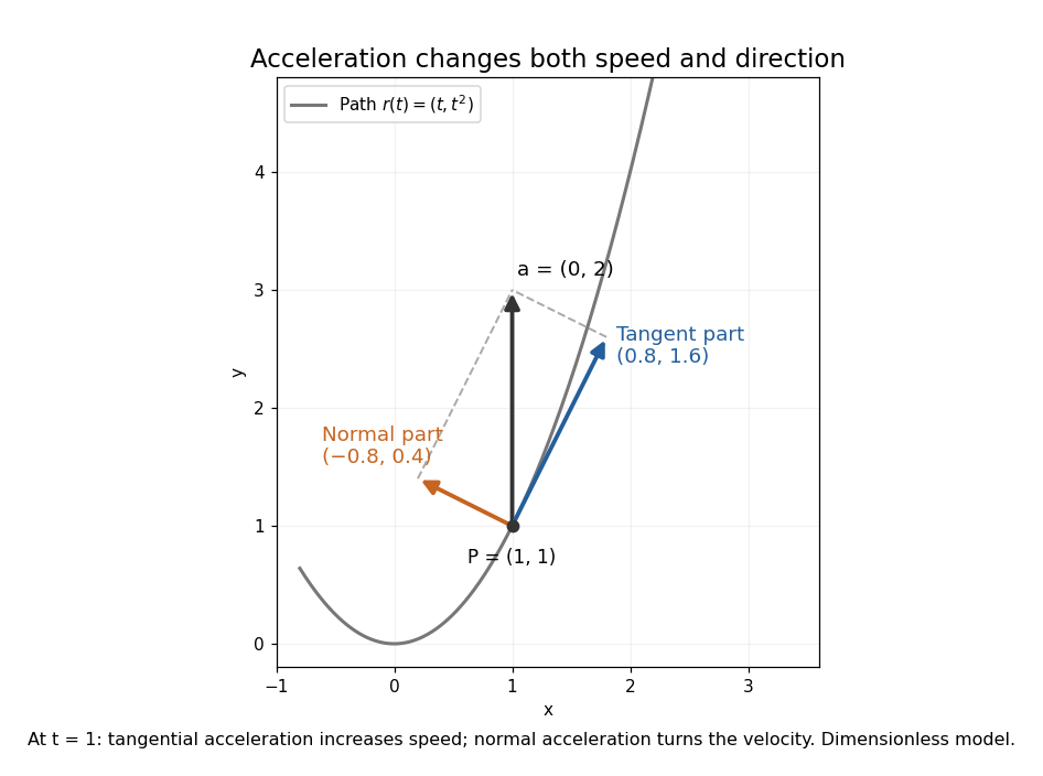
For a twice continuously differentiable regular curve describing motion, let $v=\Vert r^{\prime }(t)\Vert >0$, $T=r^{\prime }/v$, and let $N$ be the principal normal vector where the curvature $\kappa$ is positive. Differentiating the velocity vector $r^{\prime }=vT$ givesThe tangential component changes the speed; the normal component changes the direction of the velocity vector. A particle can therefore have nonzero acceleration at constant speed, as in circular motion with constant speed. The formula follows from $dT/dt=(dT/ds)(ds/dt)=\kappa vN$ and the product rule. When $\kappa =0$, the normal contribution vanishes even though the principal normal vector is undefined there. ^[ref]

In dimensionless coordinates, take $r(t)=(t,t^2)$. At $t=1$,The resulting vector components areBoth increasing speed and turning contribute to the same acceleration.

A tangent vector at a point $p$ of a smooth manifold without boundary records an instantaneous velocity through $p$. Its base point is part of the data; measuring its length additionally requires a Riemannian metric. Intrinsically, a smooth curve $\gamma$ with $\gamma (0)=p$ defines its tangent vector by how every local smooth function changes along it:This is a derivation at a point. Two smooth curves through $p$ represent the same tangent vector if these derivatives agree for every such smooth function; equivalently, their coordinate velocity vectors agree in one manifold chart. The chain rule makes that agreement independent of the chosen manifold chart. ^[ref]

For an embedded submanifold of Euclidean space, the intrinsic tangent vector is represented by the ordinary derivative ${\gamma }^{\prime }(0)$, with its base point $p$ retained. A drawn arrow starting at $p$ represents that tangent vector; its endpoint $p+{\gamma }^{\prime }(0)$ need not lie on the embedded submanifold. Nor is a tangent vector required to be a unit tangent vector: a stationary smooth curve gives the zero vector, which belongs to the tangent space but has no direction to normalize.

Here are explicit calculations. In ${\mathbb{R}}^2$, $\gamma (t)=(t,t^2)$ and $\eta (t)=(t,2t^2)$ have different routes but the same tangent vector $(1,0)$ at $(0,0)$. For $f(x,y)=3x+y$, both give $v(f)=3$. For a circle of radius $R$, $c(t)=(R\cos (\omega t),R\sin (\omega t))$ has tangent vector $(0,R\omega )$ at $(R,0)$: changing $\omega$ changes the speed or reverses travel without changing the circle.

A reparametrization $\beta (s)=\gamma (h(s))$ with $h(0)=0$ gives, by the chain rule, ${\beta }^{\prime }(0)=h^{\prime }(0){\gamma }^{\prime }(0)$. A regular change of curve parameter has $h^{\prime }(0)\ne 0$. The singular choice $h(s)=s^3$ instead givesBoth describe the same parabola, whose tangent line at the origin is still the horizontal axis. The zero velocity diagnoses this singular change of curve parameter, whose inverse is not differentiable at zero; it does not show that the geometric tangent line is absent. The regular curve $\gamma$ supplies its nonzero direction.

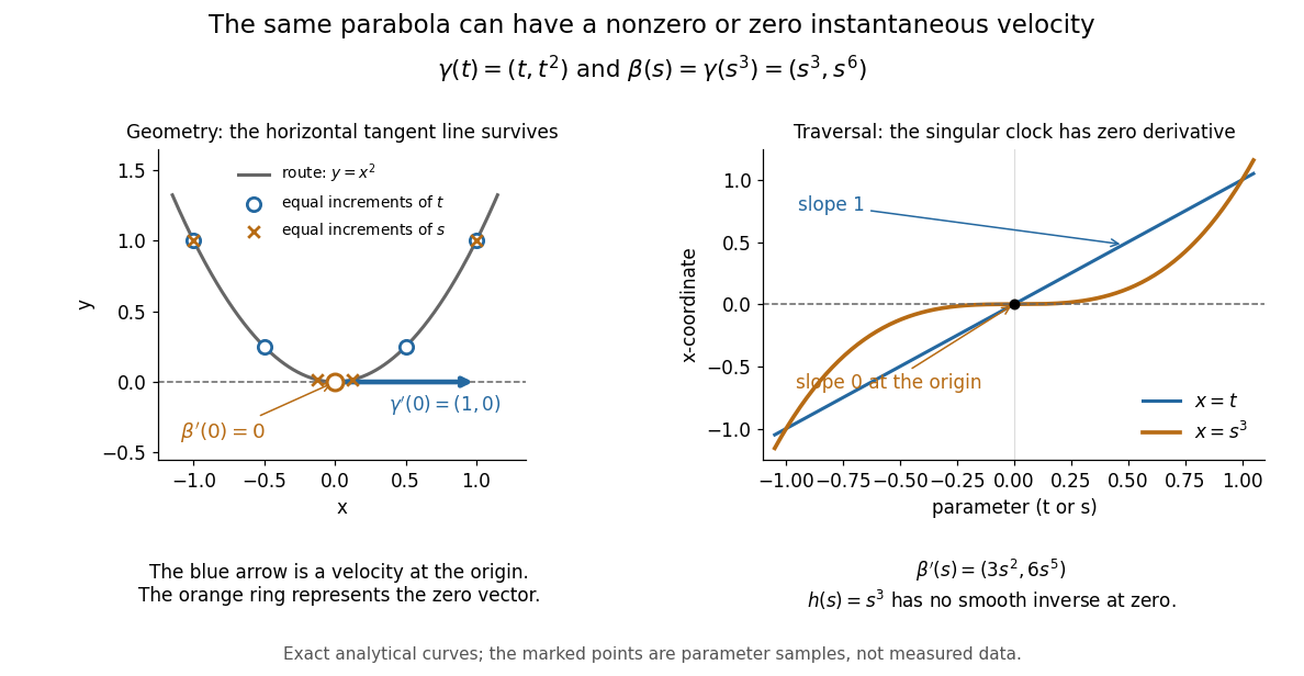
The diagram is an analytical illustration of these exact parametric curves, with equal parameter increments marked on each route. It separates geometry from traversal: the tangent line depends on the route, while a velocity vector also depends on how the curve parameter advances.

For a regular curve $\mathbf{r}(t)$ with nonzero velocity vector, its unit tangent vector isThe Euclidean norm in the denominator removes the traversal speed, leaving a unit vector that records direction. A positive change of traversal speed leaves this direction unchanged; reversing the direction of travel reverses $T$. In arc length coordinates, $T=d\mathbf{r}/ds$.

For the parabola $\mathbf{r}(t)=(t,t^2)$, the velocity vector is $(1,2t)$ and the speed is $\sqrt{1+4t^2}$. At $t=1$, $T=(1,2{)}^T/\sqrt{5}$. The tangent vector $(1,2{)}^T$ and the unit tangent vector point in the same direction, but only the latter has Euclidean norm one. The principal normal vector is a further choice based on how this direction changes, where the curvature is nonzero. ^[ref]