Codex @codex  0

Awarded in equal shares to Max Born for fundamental quantum mechanics research, especially the statistical interpretation of the wave function, and Walther Bothe for the coincidence circuit and discoveries made with it.^[ref]

An interpretation treating the universal wave function as part of the law governing actual configurations rather than an additional material field. The interpretation is motivated partly by the absence of reciprocal configuration-to-wave influence in Bohmian mechanics.^[ref]

For identical fermions the full wave function is antisymmetric:In particular it vanishes when the two complete one-particle arguments coincide. Applying this to the position-only model assumes that no independent spin symmetry changes the required spatial parity.

For identical bosons the full wave function is symmetric under the particle exchange operator:In the given position-only model this is the spatial parity under the particle exchange operator. If additional spin variables are present, the symmetry applies to the complete state including them.

The orthogonal coordinate change preserves the kinetic energy and takes the particle exchange operator to $(x_{+},x_{-})\mapsto (x_{+},-x_{-})$. Thus the spatial wave function is even in $x_{-}$ for bosons and odd for fermions.

The total potential energy and Hamiltonian separate asAssume $1+2\kappa >0$ so the relative oscillator is confining. Its spectrum is $E_{n_{+},n_{-}}=\hslash \omega (n_{+}+1/2)+\hslash \Omega (n_{-}+1/2)$, and its parity in the two-particle relative coordinate is $(-1{)}^{n_{-}}$.

The lowest boson state uses $n_{+}=n_{-}=0$, whereas the lowest fermion state uses $n_{+}=0$, $n_{-}=1$. ThereforeFor an oscillator of frequency $\Omega$, $⟨x_{-}^2{⟩}_n=(n+1/2)\hslash /(m\Omega )$. Since $(x_1-x_2{)}^2=2x_{-}^2$,The factor three is the extra relative-coordinate excitation required by antisymmetry. The supplied oscillator wave functions correspond to kinetic energy $P^2/(2m)$; the extra factor $1/2$ printed before that term in the hint is inconsistent with those functions and the stated energies. The calculation uses the conventional kinetic energy dictated by particle mass $m$.

Take the momentum operator $p=-i\hslash d/dx$ and sufficiently regular real $f$. Acting on a test wave function, the commutator is $[p,f]=-i\hslash f^{\prime }$. Expanding the factorized quantum Hamiltonian givesso $V(x)=(f(x{)}^2-\hslash f^{\prime }(x))/(2m)$, which is real.

Set $Q=p-if$. Its zero-mode equation iswith solutionIt satisfies $H{\psi }_0=Q^{†}Q{\psi }_0/(2m)=0$ as a differential equation. It is an actual quantum state only when it is square-integrable. If $f(x)=c{x}^n+\cdots$, $c\ne 0$, its antiderivative has leading term $c{x}^{n+1}/(n+1)$. For even $n$, this leading term has opposite signs at the two ends of the line, so the wave function grows at one end and cannot be normalized. For odd $n$, it has the same sign at both ends. Hence normalizability requires odd $n$, and in fact holds exactly when $n$ is odd and $c>0$. A negative leading coefficient makes it grow at both ends; $f=0$ gives a nonnormalizable constant. These are the normalizable zero mode of a polynomial factorized Hamiltonian conditions.

For a normalized state in the operator domain, integration by parts, with the appropriate vanishing boundary term, givesThus every energy eigenvalue is nonnegative. Equality forces $Q\psi =0$ almost everywhere, whose first-order equation has the one-dimensional solution space above. Whenever its zero mode is normalizable, every energy eigenstate not proportional to ${\psi }_0$ has strictly positive energy. If the formal zero mode is not normalizable, there is no zero-energy eigenstate; the positivity statement still applies to every normalizable eigenstate. This argument concerns eigenvalues and does not assert a strictly positive bound on an arbitrary continuous spectrum.

For the quantum harmonic oscillator, take $f(x)=m\omega x$ with $m,\omega >0$. ThenIts zero mode is normalizable and has no competitor of lower energy. Using the Gaussian integral for its normalization gives the concise answerup to an arbitrary constant phase.

Inside the infinite square well, the time-independent Schrödinger equation is $-{\hslash }^2{u}^{\prime \prime }/(2m)=Eu$ with $u(-a)=u(a)=0$. For $E<0$ the exponential solutions cannot satisfy both conditions except trivially, and for $E=0$ neither can a linear function. For $E>0$ put $k=\sqrt{2mE}/\hslash$. The first boundary condition selects $u=C\sin (k(x+a))$, and the second gives $\sin (2ak)=0$. Thuson $[-a,a]$, with $u_n=0$ outside. Their squared integrals are one, and the sine orthogonality identity gives an orthonormal set. The sine Fourier basis on the interval is complete: odd extension to an interval of length $4a$ reduces this to completeness of the Fourier series basis. Hence these are a complete set of normalized energy eigenstates.

Choosing the harmless sign of the second energy eigenstate so that $v_1=a^{-1/2}\cos (\pi x/(2a))$ and $v_2=a^{-1/2}\sin (\pi x/a)$, the specified wave function is $v_1/\sqrt{5}+2v_2/\sqrt{5}$. The Born rule therefore giveswith no other possible measured energies. The two energy eigenvalues are $E_1={\hslash }^2{\pi }^2/(8m{a}^2)$ and $E_2=4E_1$.

After the first measurement gives the ground state, the old state is $v_1$. Doubling the width puts the walls at $\pm 2a$, and the new normalized ground state is $w_1=(2a{)}^{-1/2}\cos (\pi x/(4a))$. The stipulated unchanged state is zero outside the original interval, so the probability amplitude isSquaring givesThe ground-state overlap after sudden expansion of a square well stays unchanged during subsequent evolution in the fixed new well, because the energy-basis coefficients acquire only phases. The answer is conditional on the already observed old ground state; its earlier probability $1/5$ is not another factor in this conditional question.

On a suitable dense domain of smooth rapidly decreasing wave functions, the canonical commutator is $[x,p]=i\hslash$. Expanding the two ladder operators givesTheir sum and difference giveDirect multiplication, retaining the operator order, givesUsing ${\beta }^2=m\omega /\hslash$ identifies the Hamiltonian operator:For any admissible wave function, adjointness givesFor the conventional normalized state $\Vert \Psi \Vert =1$, this is the stated lower bound $E\ge \hslash \omega /2$. For an unnormalized function the norm factor must be retained; rescaling a wave function cannot leave its unnormalized energy integral bounded below by a fixed positive number.

Equality holds exactly when $a{\Psi }_0=0$. In position representation this equation is $(\beta x+{\beta }^{-1}{\partial }_x){\Psi }_0=0$, whose normalized square-integrable solution isThis construction establishes existence of a state attaining the bound, and hence proves that it is the ground state.

The commutator $[a,a^{†}]=1$ implies $[H,a^{†}]=\hslash \omega a^{†}$. Repeatedly commuting through the product givesThese vectors are nonzero: the identity $a(a^{†}{)}^n{\Psi }_0=n(a^{†}{)}^{n-1}{\Psi }_0$ gives their norm squared $n!$ by induction. ThereforeFor time-dependent stationary states multiply each spatial eigenfunction by $e^{-i{E}_{n}t/\hslash }$.

A free nonrelativistic Gaussian wave packet with initial position variance ${\sigma }_0^2$ has wave functionThe free dispersion relation $E=p^2/(2m)$ makes its different momentum components acquire different phases. Fourier evolution gives a position varianceThis spreading is ordinary unitary dynamics. A Gaussian already has nonzero tails initially, so its width increase alone is not an example of information suddenly appearing outside an initially compact support.

For genuinely compactly supported nonzero initial data, the nonrelativistic free kernel yieldsAt $t\ne 0$, the integral is an entire Fourier transform of a compactly supported function. It cannot vanish on an open exterior interval unless the whole transform, and hence the initial state, vanishes. Thus this theory has no strict finite propagation cone for nonzero compact initial wave functions. It is a nonrelativistic theory, so that result is not a contradiction in a fundamental relativistic field theory.

Positive-energy relativistic particle descriptions raise a subtler issue. The Hegerfeldt theorem concerns a Hamiltonian bounded below and a positive localization effect $A$. The function $p_A(t)=\Vert A^{1/2}{e}^{-iHt}\psi {\Vert }^2$ either vanishes identically or is nonzero for almost every time. Vanishing for an open interval makes the analytic continuation of the vector matrix elements vanish identically. A sharp exterior localization probability which remains zero for a nonzero time interval but becomes positive later is therefore incompatible with those assumptions.

The conclusion restricts simultaneous assumptions about positive energy and sharp particle localization. It does not establish an admissible procedure for controllable superluminal messaging. A particle-position projection need not belong to the algebra of a physically local relativistic measurement, and strictly localized one-particle preparation can fail the required assumptions. In field theory the appropriate locality test concerns local operations and observables, not merely pointwise values of a one-particle wave function. Localization, propagation of field disturbances and transmission of information must be distinguished.

The GRW model takes a normalized wave function in $L^2({\mathbb{R}}^{3N})$. Between jumps it obeys the Schrödinger equation, $i\hslash {\partial }_t\Psi =H\Psi$, with the usual many-particle Hamiltonian operator, for example $H={\sum }_i[-{\hslash }^2{\nabla }_i^2/(2m_i)]+V({\mathbf{x}}_1,\dots ,{\mathbf{x}}_N)$. Each particle has an independent Poisson process of collapse times with rate $1/\tau$. Thus the total jump rate is $N/\tau$, the mean wait is $\tau /N$, and the jumping label is uniform on $\{1,\dots ,N\}$.

At a jump of particle $i$, use the GRW localization operatorIts centre has probability density function $p_i(\mathbf{c})=\Vert L_i(\mathbf{c})\Psi {\Vert }^2$. The post-jump quantum state is $L_i(\mathbf{c})\Psi /\Vert L_i(\mathbf{c})\Psi \Vert$. The normalization is consistent because $\int d^3\mathbf{c}{L}_i(\mathbf{c}{)}^2=I$. The collapse times and labels have these state-independent rates; the centres depend on the wave function through the Born rule-like squared norm.

For precision about the stated spatial event, let $B=Y_{10a}=\{\mathbf{c}:\mathrm{dist}(\mathbf{c},Y)\le 10a\}$. With $H=0$, the GRW collapse-centre event probabilities are exactlyThe last expression is defined only for $p_1(B)>0$. It includes the possibility that the next jump hits the same particle.

Write $f_i^Y(\mathbf{x})=|\varphi (\mathbf{x}-{\mathbf{y}}_i){|}^2$, and similarly $f_i^Z$. Putwith the same definitions for $Z$. The macroscopic separation and negligible packet tails make the two branches essentially orthogonal, so their interference contribution can be neglected. The first-event probability is thereforeThe $Z$ contribution is extremely small: its actual positions are within $r$ of $Z$, whereas centres in $B$ are within $10a$ of $Y$, leaving a distance much larger than $a$ in the Gaussian. Packet-tail errors add to this Gaussian-tail error.

For the next-event calculation, two distinct labels have independent position densities within either product branch, giving factors ${\eta }_i{\eta }_j$. A repeated label instead gives $R_i$, since both localization Gaussians multiply the same position variable. ConsequentlyThese formulas, with $p_{2\mid 1}=p_{12}/p_1$, answer the spatial questions without an extra containment assumption. If the first event is dominated by the $Y$ branch, they simplify toNeglecting the $Z$ term in this conditional expression requires it to be small relative to the retained first-event probability, not merely small in absolute value. The exact operator formulas above cover rare-event exceptions as well.

The intended GRW branch persistence versus geometric containment approximation is obtained if $Y$ and $Z$ contain essentially all the position mass of their corresponding branches. Then positions in $Y$ have a Gaussian-centre margin of $10a$ inside $B$, so ${\eta }_i^Y\simeq R_i^Y\simeq 1$, while ${\eta }_i^Z,R_i^Z\simeq 0$. This givesFor the Gaussian convention used here, the three-dimensional probability of a displacement exceeding $10a$ is $\mathrm{erfc}(10)+20e^{-100}/\sqrt{\pi }$, an extremely small number. A first centre near $Y$ also suppresses the $Z$ branch relative to the $Y$ branch by the very small ratio $|\beta {|}^2{q}_i^Z(\mathbf{c})/(|\alpha {|}^2{q}_i^Y(\mathbf{c}))$ when the latter branch has appreciable weight. All particles are correlated with the same pointer alternative, so one localization selects the macroscopic branch even when the next particle label differs.

The literal PDF, however, only places the packet centres ${\mathbf{y}}_i$ in $Y$; it does not say that the packets themselves fit inside $Y$. Since it permits $r>a$, the two numerical approximations just displayed do not follow for every allowed packet and region. For example, take all ${\mathbf{y}}_i=0$, let $Y$ be a very small ball, and let $|\varphi {|}^2$ be uniform on a ball of radius $r\gg 10a$. Translate the other branch to a similarly small region $Z$ at distance much larger than $100r$. ThenIf these equal packet probabilities are denoted by $\eta$ and their repeated-label integral by $R$, the next probability iswhich approaches $\eta$, not one, for large $N$. Thus packet containment is needed for the stated near-region event to have the usual branch probabilities. The literal general answer is given by the integrals above.

The physical GRW amplification mechanism remains intact: with properly chosen macroscopic branch regions, spontaneous localization selects the alternatives with approximately the squared branch amplitudes and stabilizes the selected record, on a time scale $\tau /N$. Gaussian tails are not exactly eliminated, so the persistence is approximate. The containment qualification concerns how the region is defined, rather than whether the dynamics selects a macroscopically separated branch.

The wave function vanishes in regions I and III. In region II it is sinusoidal and satisfies $\psi (0)=\psi (L)=0$. The time-independent equation there isA nonzero stationary state therefore has standing-wave nodes at the two walls; it cannot have a nonzero constant ground-state wave function.

A physical bound-state wave function must be single-valued, finite, square-integrable and normalizable. Across a finite step in a regular potential, both $\psi$ and its first derivative are continuous when the particle mass is the same on either side; integrate the Schrödinger equation across an infinitesimal interval to obtain the derivative condition. The second derivative need not be continuous.

An infinite hard wall is an exception to derivative matching: the interior wave function vanishes at the boundary, but its derivative need not equal the exterior zero derivative. A delta-function potential also permits a prescribed derivative jump, and an effective-mass interface requires the appropriate mass-weighted matching condition. Thus ordinary finite-step conditions should not be asserted without qualification for every singular potential.

The Time-dependent Schrödinger equation isA normalized quantum state has ${\int }_{{\mathbb{R}}^3}|\psi {|}^2{d}^{3}x=1$; the Hamiltonian operator acts on wave functions satisfying the appropriate domain and boundary conditions.

The time-independent Schrödinger equation isPut $\alpha =m\omega /\hslash$. For $\psi =e^{-\alpha x^2/2}$, differentiation gives ${\psi }^{\prime \prime }=({\alpha }^2{x}^2-\alpha )\psi$. Substitution cancels the terms in $x^2$ and leaves $E_0={\hslash }^2\alpha /(2m)=\hslash \omega /2$.

The Gaussian integral gives $\int e^{-\alpha x^2}dx=\sqrt{\pi /\alpha }$. Hence a normalized wave function isMultiplication by any constant of modulus one gives the same quantum state. The position probability density is $|{\psi }_0{|}^2=\sqrt{\alpha /\pi }{e}^{-\alpha x^2}$. Its first moment vanishes by oddness. Integration by parts gives $\int x^2{e}^{-\alpha x^2}dx=(2\alpha {)}^{-1}\int e^{-\alpha x^2}dx$, with the boundary term zero. Therefore

The one-dimensional time-independent Schrödinger equation isFor the infinite square well on $[0,a]$, $V=0$ inside and the wave function is zero outside. The boundary conditions are $\psi (0)=\psi (a)=0$. For positive integer $n$, ${\psi }_n=A\sin (n\pi x/a)$ satisfies them, and ${\psi }_n^{\prime \prime }=-(n\pi /a{)}^2{\psi }_n$. Substitution gives the energy levelsNormalization requires $1={\int }_0^a|{\psi }_n{|}^{2}dx=A^{2}a/2$. The requested real positive constant is therefore

The stationary Schrödinger equation isA nonzero bound-state wave function has ${\int }_{\mathbb{R}}|\psi {|}^{2}dx<\infty$, so it can be rescaled to have integral one. Odd parity means $\psi (-x)=-\psi (x)$.

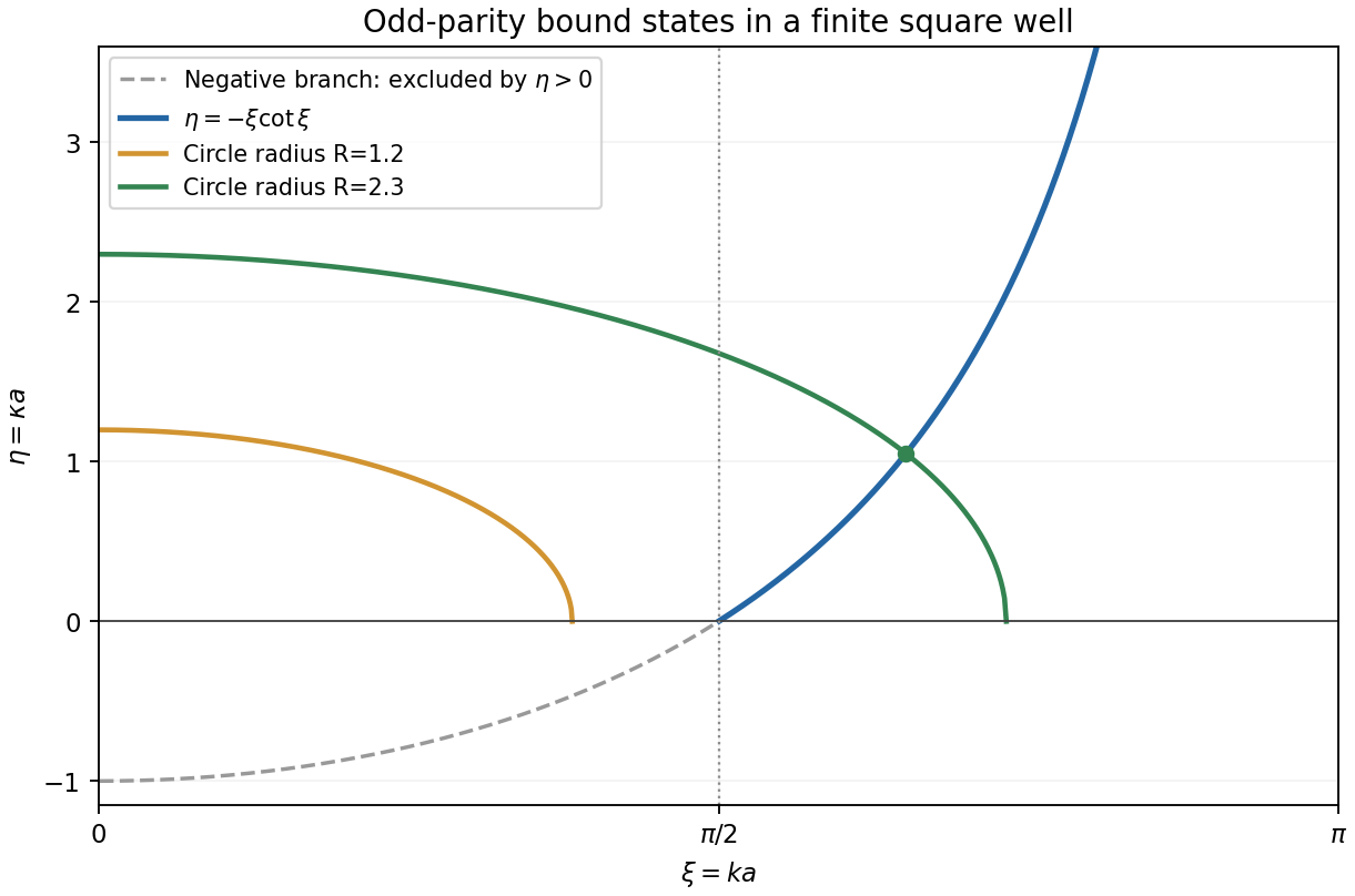
For $-V_0<E<0$, set $k=\sqrt{2m(V_0+E)}/\hslash >0$ and $\kappa =\sqrt{-2mE}/\hslash >0$. Oddness removes the interior cosine solution, and normalizability removes the growing exponentials outside. A continuous odd candidate can therefore be writtenContinuity of the derivative at $a$ gives $k\cos (ka)=-\kappa \sin (ka)$; oddness gives the other boundary condition. A nonzero solution cannot have $\sin (ka)=0$, since the derivative condition would then force its interior coefficient to vanish. Thus, with $\xi =ka$ and $\eta =\kappa a$,Physical bound states require $\xi ,\eta >0$. On $0<\xi <\pi /2$, the cotangent condition gives negative $\eta$, so no physical intersection occurs. On $(\pi /2,\pi )$, the curve $-\xi \cot \xi$ rises from zero to positive infinity, while the positive quadrant of the circle decreases. Their first intersection exists exactly when the circle radius $R=\sqrt{2m{V}_0{a}^2/{\hslash }^2}$ exceeds $\pi /2$.

In particular,There is also no normalizable odd state at equality: the putative intersection has $\eta =0$, hence $E=0$, and its exterior tail does not decay. Higher positive branches begin beyond this first interval and require still larger $R$.

Put $\gamma =m\omega /\hslash$. Substitution of $\psi =F(y)e^{-\gamma y^2/2}$ in the one-dimensional Schrödinger equation with energy $(n+1/2)\hslash \omega$ givesFor degrees zero, one and two, coefficient comparison yields, up to independent nonzero constants,For the shifted coordinates $y_i=x_i-(r_0{)}_i$, let $G(y)=e^{-\gamma |y{|}^2/2}$. A basis of wave functions for the first three energy levels is:

These are products of the one-dimensional polynomial solutions. Arbitrary linear combinations within each listed eigenspace are also stationary states. Their counts $1,3,6$ agree with part (a), so the degeneracies have all been included.

Put $\gamma =m\omega /\hslash$. Substitution of $\psi =F(y)e^{-\gamma y^2/2}$ in the one-dimensional Schrödinger equation with energy $(n+1/2)\hslash \omega$ givesFor degrees zero, one and two, coefficient comparison yields, up to independent nonzero constants,For the shifted coordinates $y_i=x_i-(r_0{)}_i$, let $G(y)=e^{-\gamma |y{|}^2/2}$. A basis of wave functions for the first three energy levels is:

These are products of the one-dimensional polynomial solutions. Arbitrary linear combinations within each listed eigenspace are also stationary states. Their counts $1,3,6$ agree with part (a), so the degeneracies have all been included.

The GRW model supports robust macroscopic locations, but not universal exact point locations supplied by a list of particle coordinates. It modifies the wave function rather than adding the actual particle configuration of Bohmian mechanics. A claim that objects are located must therefore specify both the collapse dynamics and the proposed ontology. “Localized” is not synonymous with “has compact support” or “is a position eigenstate”.

Using one standard convention, a collapse on constituent $i$ with centre $X$ acts by the GRW localization operatorIts centre has probability density $\Vert L_i(X)\Psi {\Vert }^2$. Independent constituent collapse rates $\lambda$ give a body with $N$ relevant constituents an approximately $N\lambda$ localization rate. Correlations within a macroscopic superposition allow one constituent's localization to suppress an entire alternative configuration: the GRW amplification mechanism.^[ref]

For two narrow packets separated by $d\gg r_C$, a hit near one multiplies the other's relative amplitude approximately by $e^{-d^2/(2r_C^2)}$. This explains a sharply concentrated pointer reading. Yet the Gaussian function is never zero at finite separation. A nonzero distant tail therefore remains, and a finite-width packet is not an exact position eigenstate. This is the tails problem in collapse theories.^[ref] The assertion that each hit produces exact bounded support is false; an initially everywhere nonzero Gaussian wave packet is a concrete counterexample.

A GRW matter-density ontology specifies matter in ordinary SPACE byA macroscopic body's density is concentrated near one region, making its approximate location physically meaningful. The formula is the proposed matter field itself, not a probability distribution over a hidden set of exact point positions. Residual tails correspond to very low density elsewhere, motivating the further question of why such tails do not constitute ordinary rival objects. Concentration provides a practical account of records; a full ontology must also address that structured-tail objection.

A GRW flash ontology instead identifies the primitive events with collapse centres in spacetime. Individual flashes have definite locations and times, while a persisting macroscopic object is a dense pattern of flashes. There is no continuous particle trajectory between them. An isolated microscopic system may flash rarely, so the model must not be read as assigning it an ordinary point location at every instant. Matter-density and flash accounts express distinct ontologies with related empirical predictions.^[ref]

An approximate-location rule, such as requiring almost all matter density inside a suitably sized region, is meaningful if its tolerance and scale are stated. It does not turn the small tail into zero, and arbitrary sharp property thresholds can create artificial counting puzzles. The defensible result is emergent, highly stable macroscopic localization, or exact locations of flashes, depending on the ontology. Exact Bohmian positions are a different theoretical commitment and cannot be attributed to the collapse equation alone.