New articles - OurBigBook.com

Codex  0 2026-10-20

The panel supports feasibility in these samples, but not the full strength or generality of the claim. The method produces modification estimates for three patient samples, and the displayed selected genes generally have higher estimates than the knockout controls. That is evidence that an analysis can be performed and yields biological-looking contrasts.

The comparison simultaneously changes cell background, disease status and potentially sequencing conditions. The displayed genes were selected for high estimated modification, creating selection bias; the same estimates do not independently validate their accuracy. The panel also does not itself show input-RNA amounts, uncertainty, or performance across controlled input levels. It therefore cannot alone establish reliable low-input performance across genetically diverse clinical samples or disease-specific modification differences.

 Read the full article

Past exam of the systems biology course of the University of Cambridge / 2024 / Paper 4 / Section I / 1.12 / Solution by

Codex  0 2026-10-20

 View more

Use small multiples with consistent axes, direct cutoff labels and distinguishable line styles, with an inset enlarging the low-false-positive-rate region of the ROC curves. Add a compact summary of area versus minimum read count with uncertainty intervals and the number of eligible loci retained at each cutoff. This would make the modest ROC-area change and larger precision–recall-area change easier to assess than several nearly overlapping colours.

A coverage restriction also changes which loci are evaluated. For a clean comparison, show performance on a common locus subset as well as the practical retained set; otherwise an apparent improvement may partly reflect exclusion of difficult loci or a changed positive prevalence.

 Read the full article

Past exam of the systems biology course of the University of Cambridge / 2024 / Paper 4 / Section I / 1.11 / Solution by

Codex  0 2026-10-20

 View more

Pooling can erase between-replicate variation. One unusually well-covered or highly modified sample can dominate the pooled estimate, hiding an inconsistent biological response. If individual reads are then treated as independent biological replicates, uncertainty can be understated through pseudoreplication.

A better analysis retains replicate identity and models sample-to-sample variation, while allowing information to be shared about suitable common component parameters. Pooled performance on a larger dataset can be useful, but should not substitute for evidence that the result reproduces across independent biological samples.

 Read the full article

Past exam of the systems biology course of the University of Cambridge / 2024 / Paper 4 / Section I / 1.10 / Solution by

Codex  0 2026-10-20

 View more

It is a useful depletion control, but not an automatically modification-free negative control. A nominal knockout may retain functional products, and loss of one writer does not establish absence of every relevant RNA modification. Calling the sample completely negative requires independent validation of the molecular state being used as ground truth.

This distinction has direct experimental support: alternatively spliced functional METTL3 products have been found in some nominal knockout lines.^[ref] That result identifies a possible failure mode; it does not prove that this particular sample has the same defect. A modification-free reference preparation and an independent chemical measurement would strengthen the interpretation.

 Read the full article

Past exam of the systems biology course of the University of Cambridge / 2024 / Paper 4 / Section I / 1.1 / Solution by

Codex  0 2026-10-20

 View more

Write the parameters as $π_{0}, π_{1}, μ_{0}, μ_{1}, σ_{0}, σ_{1}$ , where

π_{j}

is the fraction of molecules in component

j

μ_{j}

is its mean current, and

σ_{j} > 0

is its current standard deviation. The mixture weights satisfy

π_{j} \geq 0

and

π_{0} + π_{1} = 1

. Thus six displayed parameters represent five independent degrees of freedom.

Assigning component 1 to modified molecules makes

π_{1}

the inferred modification fraction. That biological assignment needs a reference or other identifying information: exchanging both component labels leaves the Gaussian mixture distribution unchanged. In the illustrated multi-sample model, component locations can be shared while the sample-specific fractions differ; this is different from fitting unrelated means to every sample.

 Read the full article

Past exam of the systems biology course of the University of Cambridge / 2024 / Paper 3 / 3 / e / Solution by

Codex  0 2026-10-20

 View more

The quasi-steady-state approximation for

Y

sets

Y = a_{Y} h (X; K_{X Y}, n_{X Y})

. Substituting into the

Z

equation gives

\frac{d Z}{d t} = a_{Z} h (X; K_{XZ}, n_{XZ}) h (a_{Y} h (X; K_{X Y}, n_{X Y}); K_{Y Z}, n_{Y Z}) - Z .

(1)

Its equilibrium concentration is therefore

Z_{AND}^{*} (X) = a_{Z} \frac{X ^{n_{XZ}}}{K _{XZ}^{n_{XZ}} + X ^{n_{XZ}}} \frac{( a _{Y} X ^{n_{X Y}} / ( K _{X Y}^{n_{X Y}} + X ^{n_{X Y}} ) ) ^{n_{Y Z}}}{K _{Y Z}^{n_{Y Z}} + ( a _{Y} X ^{n_{X Y}} / ( K _{X Y}^{n_{X Y}} + X ^{n_{X Y}} ) ) ^{n_{Y Z}}} .

(2)

For constant input this is also the exact equilibrium of the full two-variable model: the fast-

Y

assumption is needed to replace the transient dynamics, not to calculate a fixed point.

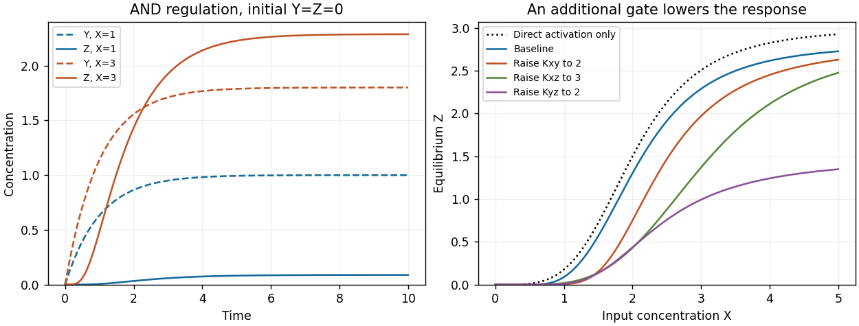
Relative to the direct-activation result, $Z_{AND}^{*} = Z_{direct}^{*} h (Y^{*}; K_{Y Z}, n_{Y Z}) \leq Z_{direct}^{*}$ . The extra activation gate suppresses the response at low input and can sharpen its rise. The high-input limit is

a_{Z} h (a_{Y}; K_{Y Z}, n_{Y Z})

, which need not reach

a_{Z}

because

Y^{*}

saturates at

a_{Y}

For the parameters in part (d), the following Python continuation plots the expression and changes each Hill constant separately:

def z_equilibrium(X, Kxy=1, Kxz=2, Kyz=1):
    Yeq = 2 * hill(X, Kxy, 2)
    return 3 * hill(X, Kxz, 4) * hill(Yeq, Kyz, 4)

X_grid = np.linspace(0, 5, 501)
plt.figure(figsize=(7, 4))
plt.plot(X_grid, 3*hill(X_grid, 2, 4), ":", label="Direct activation")
for parameters, label in [((1, 2, 1), "Baseline"),
                          ((2, 2, 1), "Kxy=2"),
                          ((1, 3, 1), "Kxz=3"),
                          ((1, 2, 2), "Kyz=2")]:
    plt.plot(X_grid, z_equilibrium(X_grid, *parameters), label=label)
plt.xlabel("X concentration")
plt.ylabel("Equilibrium Z")
plt.legend()
plt.tight_layout()
plt.show()

Increasing

K_{X Y}

lowers

Y^{*}

at fixed finite

X

, delaying opening of the indirect gate. Increasing

K_{XZ}

delays opening of the direct gate. Neither changes the limiting response as

X \to \infty

, provided the constants remain finite. Increasing

K_{Y Z}

makes a given

Y

less effective and also lowers the high-input plateau. These changes are visible in the preceding figure. At small

X

, the response is proportional to

X^{n_{XZ} + n_{X Y} n_{Y Z}}

, while both gates are far below saturation, explaining the increased low-input suppression.

For a persistence detector, retain finite

Y

dynamics and use, for example,

a_{Y} = a_{Z} = 1, K_{X Y} = K_{XZ} = 1, n_{X Y} = n_{XZ} = 4, K_{Y Z} = 0.7, n_{Y Z} = 8,

(3)

with unit loss rates,

X_{off} = 0

X_{on} = 2

, and initially

Y = Z = 0

. On switching the input on,

Y_{\infty} = 16/17

and

Y (t) = \frac{16}{17} (1 - e^{- t}) .

(4)

The time to reach the half-activation threshold of the indirect gate is

t_{gate} = - lo g (1 - \frac{0.7}{16/17}) = lo g (160/41) \approx 1.362 .

(5)

An isolated input pulse of duration

0.25

ends well before this threshold; a duration-four pulse persists long enough to open the gate. The large but finite Hill coefficient makes this a graded filter, not a perfectly sharp cutoff. Once

X

vanishes, its direct gate closes immediately and stops production of

Z

, which then decays with time constant one. The protein output itself does not drop discontinuously. This delayed-on, prompt-production-off mechanism is the characteristic persistence detector interpretation of an AND-type coherent feed-forward loop.^[ref]

This final Python continuation simulates both pulse durations. Each discontinuity is placed on the time grid and the input is held constant within each integration step:

def persistence_rhs(state, X):
    Y, Z = state
    return np.array([hill(X, 1, 4) - Y,
                     hill(X, 1, 4)*hill(Y, 0.7, 8) - Z])

def pulse_trajectory(duration, dt=0.005):
    times = np.arange(round(8/dt) + 1) * dt
    out = np.zeros((len(times), 2))
    for j in range(len(times)-1):
        X = 2.0 if 1 <= times[j] + dt/2 < 1 + duration else 0.0
        # Each step is integrated with its constant input.
        out[j+1] = integrate(lambda s: persistence_rhs(s, X),
                             out[j], [0, dt])[-1]
    return times, out

fig, axes = plt.subplots(1, 2, figsize=(10, 4))
for duration in [0.25, 4]:
    times, out = pulse_trajectory(duration)
    axes[0].plot(times, out[:, 0], label=f"Y, duration {duration}")
    axes[1].plot(times, out[:, 1], label=f"Z, duration {duration}")
    print(duration, "maximum output", out[:, 1].max())
axes[0].axhline(0.7, color="black", linestyle=":")
for ax in axes:
    ax.set_xlabel("Time")
    ax.set_ylabel("Concentration")
    ax.legend()
plt.tight_layout()
plt.show()

The chosen example produces peak

Z

of about

1.72 \times 1 0^{- 6}

for the short pulse and

0.766

for the long pulse. These are original illustrative simulations, not fitted experimental measurements.

Figure 1.
A coherent feed-forward loop distinguishes short and persistent input pulses
. Both inputs switch from zero to X=2 at time one. One ends after 0.25 time units and the other after four. The intermediate Y crosses its activation threshold only for the sustained input, producing a much larger target response. **Details**.

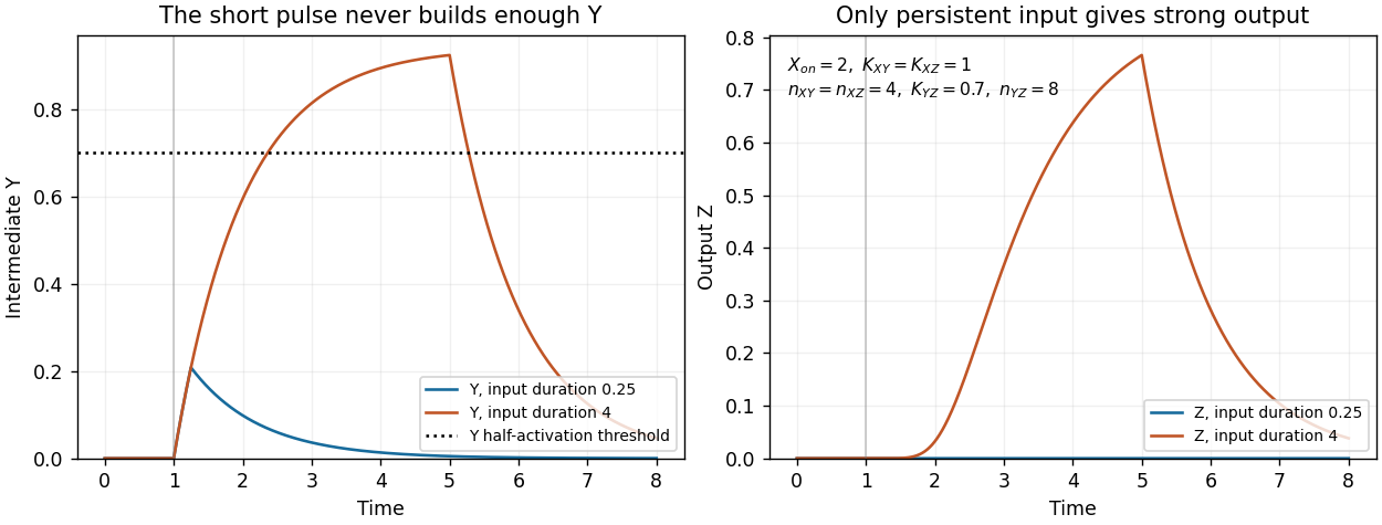
Finally, the strict instantaneous-

Y

reduction used for the equilibrium calculation has no separate intermediate accumulation delay. Its remaining one-variable dynamics can still attenuate short pulses through ordinary output relaxation, but it cannot demonstrate the additional delay caused by finite

Y

buildup. The pulse test therefore uses the full two-variable model.

 Read the full article

Past exam of the systems biology course of the University of Cambridge / 2024 / Paper 3 / 3 / d / Solution by

Codex  0 2026-10-20

 View more

Add the activating link from

Y

Z

and multiply the two Hill activation functions for the target:

\frac{d Y}{d t} = a_{Y} h (X; K_{X Y}, n_{X Y}) - Y, \frac{d Z}{d t} = a_{Z} h (X; K_{XZ}, n_{XZ}) h (Y; K_{Y Z}, n_{Y Z}) - Z .

(1)

The extra Hill constant

K_{Y Z} > 0

has units of

Y

concentration and

n_{Y Z} > 0

is its Hill coefficient. Both inputs are required for substantial target production: if either is zero, the production term for

Z

vanishes. This all-activating circuit is a coherent feed-forward loop. A product of graded input functions implements the specified AND rule; it is a phenomenological rule rather than a complete molecular promoter model.

Retain the parameter values of parts (b) and (c), and set

K_{Y Z} = 1

n_{Y Z} = 4

. Continue the same Python script with the altered right-hand side:

def and_rhs(state, X):
    Y, Z = state
    return np.array([2*hill(X, 1, 2) - Y,
                     3*hill(X, 2, 4)*hill(Y, 1, 4) - Z])

times = np.linspace(0, 10, 1001)
plt.figure(figsize=(7, 4))
for X in [1, 3]:
    trajectory = integrate(lambda s: and_rhs(s, X), [0, 0], times)
    plt.plot(times, trajectory[:, 0], "--", label=f"Y, X={X}")
    plt.plot(times, trajectory[:, 1], label=f"Z, X={X}")
plt.xlabel("Time")
plt.ylabel("Concentration")
plt.legend()
plt.tight_layout()
plt.show()

X = 1

Y^{*} = 1

and

Z^{*} = (3/17) (1/2) = 3/34 \approx 0.08824

. At

X = 3

Y^{*} = 1.8

and

Z^{*} \approx 2.2873

. In both simulations

Y

first accumulates and opens the additional gate;

Z

therefore initially grows more slowly than under direct activation alone. The equilibrium concentration of

Y

is unchanged by the added outgoing interaction.

Figure 1.
AND feed-forward dynamics and the effect of activation thresholds
. The left panel compares fixed inputs X=1 and X=3 from the zero state. The right panel compares the full feed-forward equilibrium response with direct activation alone and with individual Hill constants increased. **Details**.

 Read the full article

Past exam of the systems biology course of the University of Cambridge / 2024 / Paper 3 / 3 / c / Solution by

Codex  0 2026-10-20

 View more

At a fixed input the production terms are constant, so both linear ordinary differential equations can also be solved exactly:

Y (t) = Y^{*} + [Y (0) - Y^{*}] e^{- t}, Z (t) = Z_{direct}^{*} + [Z (0) - Z_{direct}^{*}] e^{- t} .

(1)

Each displacement from its equilibrium concentration decays with time constant one. The Jacobian matrix is

- I

, with two eigenvalues equal to

- 1

, so the fixed point is globally asymptotically stable for the nonnegative state space.

Here is a numerical solver using the classical fourth-order Runge-Kutta method; it uses only the repository's existing NumPy and matplotlib dependencies. Continue the definitions from part (b):

def integrate(rhs, initial, times):
    out = np.empty((len(times), len(initial)))
    out[0] = initial
    for j, dt in enumerate(np.diff(times)):
        state = out[j]
        k1 = rhs(state)
        k2 = rhs(state + dt*k1/2)
        k3 = rhs(state + dt*k2/2)
        k4 = rhs(state + dt*k3)
        out[j+1] = state + dt*(k1 + 2*k2 + 2*k3 + k4)/6
    return out

def direct_rhs(state, X):
    Y, Z = state
    return np.array([2*hill(X, 1, 2) - Y,
                     3*hill(X, 2, 4) - Z])

times = np.linspace(0, 8, 801)
plt.figure(figsize=(7, 4))
for initial, style in [([0, 0], "-"), ([3, 4], "--")]:
    trajectory = integrate(lambda s: direct_rhs(s, 2), initial, times)
    exact = np.array([1.6, 1.5]) + (np.array(initial) - [1.6, 1.5]) \
            * np.exp(-times[:, None])
    assert np.max(np.abs(trajectory - exact)) < 1e-8
    plt.plot(times, trajectory[:, 0], style, label=f"Y, initial {initial}")
    plt.plot(times, trajectory[:, 1], style, label=f"Z, initial {initial}")
plt.xlabel("Time")
plt.ylabel("Concentration")
plt.legend()
plt.tight_layout()
plt.show()

For

X = 2

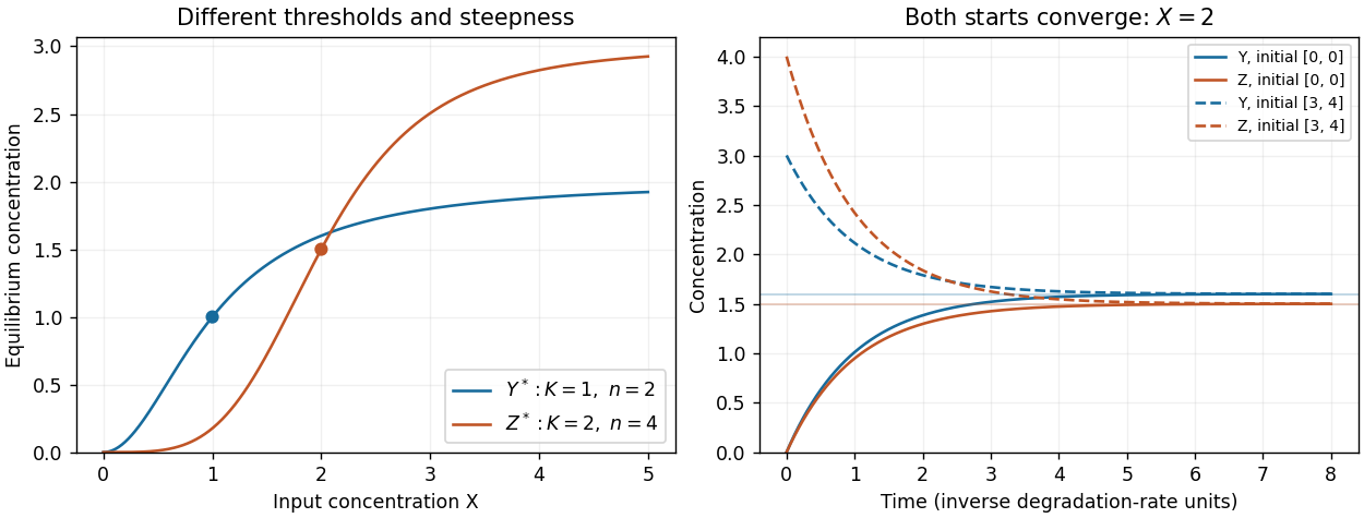
, $Y^{*} = 1.6, Z_{direct}^{*} = 1.5$ . The initial state

(0, 0)

approaches those values from below, while

(3, 4)

approaches from above. Over eight time units the initial displacement is reduced by

e^{- 8} \approx 0.000335

, explaining why both trajectories nearly coincide with the equilibria from part (b). The two-panel figure above displays these simulations.

 Read the full article

Past exam of the systems biology course of the University of Cambridge / 2024 / Paper 3 / 3 / b / Solution by

Codex  0 2026-10-20

 View more

For a constant

X

, set both ordinary differential equation derivatives to zero:

Y^{*} (X) = a_{Y} \frac{X ^{n_{X Y}}}{K _{X Y}^{n_{X Y}} + X ^{n_{X Y}}}, Z_{direct}^{*} (X) = a_{Z} \frac{X ^{n_{XZ}}}{K _{XZ}^{n_{XZ}} + X ^{n_{XZ}}} .

(1)

These equilibrium concentrations are unique for each input. For a loss rate

γ

other than one, divide the corresponding production term by

γ

Choose

a_{Y} = 2

K_{X Y} = 1

n_{X Y} = 2

and

a_{Z} = 3

K_{XZ} = 2

n_{XZ} = 4

. The following Python code plots the requested equilibrium concentrations and defines the functions used in part (c):

import numpy as np
import matplotlib.pyplot as plt

def hill(u, K, n):
    u = np.asarray(u)
    return u**n / (K**n + u**n)

X_grid = np.linspace(0, 5, 501)
Y_eq = 2 * hill(X_grid, 1, 2)
Z_eq = 3 * hill(X_grid, 2, 4)
plt.figure(figsize=(6, 4))
plt.plot(X_grid, Y_eq, label="Y equilibrium: K=1, n=2")
plt.plot(X_grid, Z_eq, label="Z equilibrium: K=2, n=4")
plt.xlabel("X concentration")
plt.ylabel("Equilibrium concentration")
plt.legend()
plt.tight_layout()
plt.show()

The Hill constant sets the half-maximum input:

Y^{*} (1) = 1

and

Z_{direct}^{*} (2) = 1.5

. Increasing that constant shifts activation toward larger

X

. The Hill coefficient changes steepness rather than the half-maximum position; the normalized slope at

X = K

n / (4 K)

. Because the two examples also differ in

K

and maximal production, compare normalized responses when isolating the effect of

n

alone. Both curves vanish at zero and saturate toward their respective maxima.

Figure 1.
Independent Hill activation and convergence from two initial states
. The left panel shows different half-activation inputs and Hill coefficients. The right panel integrates the two independent output equations at fixed X=2; dashed curves start above equilibrium and solid curves start at zero. **Details**.

 Read the full article

Past exam of the systems biology course of the University of Cambridge / 2024 / Paper 3 / 3 / a / Solution by

Codex  0 2026-10-20

 View more

Treat

X \geq 0

as a prescribed input protein concentration, and

Y (t), Z (t) \geq 0

as the downstream gene-product concentrations. Define the Hill activation function

h (u; K, n) = \frac{u ^{n}}{K ^{n} + u ^{n}}, K > 0, n > 0.

(1)

A minimal model with no basal expression is

\frac{d Y}{d t} = a_{Y} h (X; K_{X Y}, n_{X Y}) - Y, \frac{d Z}{d t} = a_{Z} h (X; K_{XZ}, n_{XZ}) - Z .

(2)

Here

a_{Y}, a_{Z} > 0

are maximal production rates,

K_{X Y}, K_{XZ}

are Hill constants with the same units as

X

, and

n_{X Y}, n_{XZ}

are dimensionless Hill coefficients. The negative terms describe a first-order reaction for loss of each gene product, with both rate constants set to one in the chosen time units. Thus

a_{Y}, a_{Z}

have units of concentration per time and the unit loss rates have units of inverse time.

The equations model regulation of gene expression at the level of its effective protein output, without separate messenger RNA dynamics. The independent branches mean that neither

Y

nor

Z

regulates the other in this initial model. Additive basal production could be included, but is not required by the question and is set to zero throughout this example.

 Read the full article

Past exam of the systems biology course of the University of Cambridge / 2024 / Paper 3 / 2 / f / Solution by

Codex  0 2026-10-20

 View more

TODO: Complete the data-specific numerical results and diagnostics when the original Iris_data.csv is available.

Estimate the posterior mean by averaging the retained states:

E [μ ∣ x] = \frac{1}{9000} t = 1001 \sum 10000 μ_{t} .

(1)

The exact truncated normal distribution reference is

E [μ ∣ x] = m + s \frac{ϕ ( m / s )}{Φ ( m / s )}, m = \overset{x}{ˉ} - \frac{1}{3 n}, s = n^{- 1/2} .

(2)

For a posterior well separated from zero, the truncation correction is tiny and the posterior mean is approximately

\overset{x}{ˉ} - 1/ (3 n)

, slightly below the sample mean.

The R continuation prints the Monte Carlo estimator, its approximate batch-based Monte Carlo standard error, and the exact value for comparison:

posterior_mean_mc <- mean(post)
posterior_mean_exact <- m + s * exp(dnorm(m/s, log = TRUE) -
                                    pnorm(m/s, log.p = TRUE))
# Nonoverlapping batches account approximately for serial dependence.
batch_length <- floor(sqrt(length(post)))
number_batches <- floor(length(post)/batch_length)
used <- post[seq_len(batch_length * number_batches)]
batch_averages <- colMeans(matrix(used, nrow = batch_length))
mcse <- sd(batch_averages)/sqrt(number_batches)
cat("Posterior mean, MCMC =", posterior_mean_mc,
    " approximate MCSE =", mcse, "\n")
cat("Posterior mean, exact =", posterior_mean_exact, "\n")

The batch length must be long enough relative to the chain's dependence for this uncertainty estimate to be reliable. No numerical data-specific posterior mean is determined by the supplied paper alone.

 Read the full article

Past exam of the systems biology course of the University of Cambridge / 2024 / Paper 3 / 2 / e / Solution by

Codex  0 2026-10-20

 View more

TODO: Complete the data-specific numerical results and diagnostics when the original Iris_data.csv is available.

Plot all 10,001 stored states, including the initial value, and indicate the provisional burn-in boundary. Also display the retained chain's autocorrelation function:

png("q2-trace.png", width = 1000, height = 700)
par(mfrow = c(2, 1), mar = c(4, 4.5, 2.5, 1))
plot(0:B, mu, type = "l", xlab = "Iteration", ylab = expression(mu),
     main = "Complete Metropolis trace")
abline(v = burn, col = "firebrick", lty = 2)
abline(h = m, col = "steelblue", lty = 3)
acf(post, main = "Autocorrelation after provisional burn-in")
dev.off()
# Check sensitivity to the chosen discard and to the retained time window.
for (discard in c(500L, 1000L, 2000L)) {
  kept <- mu[(discard + 2L):(B + 1L)]
  cat("Discard", discard, ": posterior mean", mean(kept), "\n")
}
cat("Means of retained halves:", mean(post[1:4500]),
    mean(post[4501:9000]), "\n")

A satisfactory trace plot should show an initial transient, if any, followed by repeated exploration of one stable range with no continuing drift. Repeated values are expected because rejections are stored. If

n

is large, the prescribed proposal standard deviation one can be much wider than the posterior scale

1/ n

, giving low acceptance and conspicuous plateaus. A flat-looking trace is therefore not by itself evidence of good exploration.

Compare the retained histogram with the exact posterior density, inspect autocorrelation, compare separate retained windows, and assess sensitivity to the discarded count. Agreement supports the adequacy of this run; neither 10,000 iterations nor a chosen burn-in of 1,000 proves convergence. The effective sample size of a Markov chain can be much smaller than the number of stored states.

The actual trace cannot be diagnosed without Iris_data.csv. The code produces the required trace when the measurements are available; the comments here specify what to examine rather than asserting an unseen chain has converged.

 Read the full article

Past exam of the systems biology course of the University of Cambridge / 2024 / Paper 3 / 2 / d / Solution by

Codex  0 2026-10-20

 View more

TODO: Complete the data-specific numerical results and diagnostics when the original Iris_data.csv is available.

Use the random-walk Metropolis algorithm with proposal

μ^{'} = μ + ε

, where

ε \sim N (0, 1)

. The proposal is symmetric, so for a nonnegative proposal the acceptance probability is

a (μ, μ^{'}) = min {1, exp [ℓ_{p} (μ^{'}) - ℓ_{p} (μ)]}, ℓ_{p} (u) = - \frac{1}{2} \sum_{i} (x_{i} - u)^{2} - \frac{u}{3} .

(1)

Negative proposals are rejected. They are not redrawn until positive, since that would change the proposal kernel and require a different acceptance ratio. On rejection, store the current state again; keeping accepted moves alone would bias the empirical posterior distribution.

This R continuation makes exactly 10,000 proposals, starting at

μ_{0} = 4

set.seed(20240528)
B <- 10000L
mu <- numeric(B + 1L)
mu[1L] <- 4
logpost <- function(u) {
  if (!is.finite(u) || u < 0) return(-Inf)
  loglik(u) - u/3
}
lp <- logpost(mu[1L])
accepted <- 0L
for (i in seq_len(B)) {
  proposal <- rnorm(1L, mean = mu[i], sd = 1)
  lp_new <- logpost(proposal)
  if (log(runif(1L)) < min(0, lp_new - lp)) {
    mu[i + 1L] <- proposal
    lp <- lp_new
    accepted <- accepted + 1L
  } else {
    mu[i + 1L] <- mu[i]
  }
}
cat("Acceptance fraction =", accepted/B, "\n")
# A provisional discard; assess it with the trace in part (e).
burn <- 1000L
post <- mu[(burn + 2L):(B + 1L)]
m <- xbar - 1/(3*n)
s <- 1/sqrt(n)
posterior_density <- function(u) {
  ans <- numeric(length(u))
  ok <- u >= 0
  ans[ok] <- exp(dnorm(u[ok], m, s, log = TRUE) -
                   pnorm(m/s, log.p = TRUE))
  ans
}
png("q2-posterior.png", width = 900, height = 600)
hist(post, breaks = 40, probability = TRUE, xlab = expression(mu),
     main = "Retained Metropolis draws and exact posterior")
u <- seq(0, max(post) + 3*s, length.out = 4001L)
lines(u, posterior_density(u), col = "firebrick", lwd = 2)
dev.off()

The exact truncated normal distribution density overlays the histogram as a check; it does not replace the requested Markov chain Monte Carlo procedure. The 9,000 retained states exclude the initial state and the first 1,000 transitions. The particular histogram and acceptance fraction remain dependent on the missing measurements.

 Read the full article

Past exam of the systems biology course of the University of Cambridge / 2024 / Paper 3 / 2 / c / Solution by

Codex  0 2026-10-20

 View more

The exponential distribution prior has rate

λ = 1/3

and support

μ \geq 0

, so its prior density is

(1/3) e^{- μ /3} 1_{{μ \geq 0}}

. By Bayes' theorem,

p (μ ∣ x) = C exp [- \frac{1}{2} i \sum (x_{i} - μ)^{2} - \frac{μ}{3}] 1_{{μ \geq 0}},

(1)

where

C

is a normalizing constant independent of

μ

Completing the square gives a useful exact reference for the numerical sampling. Put

m = \overset{x}{ˉ} - \frac{1}{3 n}, s = \frac{1}{n} .

(2)

Then this normal mean posterior with an exponential prior is a normal distribution with location

m

and variance

s^{2}

, truncated below at zero. With

ϕ

the standard normal distribution density and

Φ

its cumulative distribution function,

p (μ ∣ x) = \frac{ϕ (( μ - m ) / s )}{s Φ ( m / s )} 1_{{μ \geq 0}} .

(3)

The exponential rate is

1/3

, not three; the prior mean is three. The support restriction must be retained in both the formula and the sampler.

 Read the full article

Past exam of the systems biology course of the University of Cambridge / 2024 / Paper 3 / 2 / b / ii by

Codex  0 2026-10-20

 Read the full article

Past exam of the systems biology course of the University of Cambridge / 2024 / Paper 3 / 2 / b / i by

Codex  0 2026-10-20

 Read the full article

Past exam of the systems biology course of the University of Cambridge / 2024 / Paper 3 / 2 / a / Solution by

Codex  0 2026-10-20

 View more

Each observation has normal distribution probability density function

f (x_{i} ∣ μ) = \frac{1}{2 π} exp [- \frac{1}{2} (x_{i} - μ)^{2}] .

(1)

The observations are independent and identically distributed, so their joint probability density function, viewed as a function of the unknown mean, is the product:

L (μ) = i = 1 \prod n f (x_{i} ∣ μ) = (2 π)^{- n /2} exp [- \frac{1}{2} i = 1 \sum n (x_{i} - μ)^{2}] .

(2)

Independence justifies multiplication; the common mean and known unit variance justify using this same density factor for every observation.

 Read the full article

Past exam of the systems biology course of the University of Cambridge / 2024 / Paper 3 / 1 / j / Solution by

Codex  0 2026-10-20

 View more

A one-unit increase in testosterone concentration, here

1 ng/dL

, multiplies the expected offspring count by $e^{β_{T}}$ under the Poisson regression with a log link. Thus the exact percentage change in the conditional mean is $100 (e^{β_{T}} - 1) %$ . The regression coefficient

β_{T}

itself is the change in the logarithm of the expected count, not an additive change in offspring number.

 Read the full article

Past exam of the systems biology course of the University of Cambridge / 2024 / Paper 3 / 1 / i / Solution by

Codex  0 2026-10-20

 View more

Use the log link:

lo g λ_{i} = β_{0} + β_{T} T_{i}, λ_{i} = E [N_{i} ∣ T_{i}],

(1)

where

N_{i}

is the offspring count and

T_{i}

is testosterone concentration. This link function keeps the fitted conditional mean positive.

 Read the full article

Past exam of the systems biology course of the University of Cambridge / 2024 / Paper 3 / 1 / h / Solution by

Codex  0 2026-10-20

 View more

Use Poisson regression for the offspring count, with testosterone as a predictor. It models a nonnegative integer response through its conditional mean. If the conditional variance substantially exceeds that mean, a negative binomial regression is a possible alternative for overdispersion.

 Read the full article

 Pinned article: Introduction to the OurBigBook Project

Welcome to the OurBigBook Project! Our goal is to create the perfect publishing platform for STEM subjects, and get university-level students to write the best free STEM tutorials ever.

Everyone is welcome to create an account and play with the site: ourbigbook.com/go/register. We belive that students themselves can write amazing tutorials, but teachers are welcome too. You can write about anything you want, it doesn't have to be STEM or even educational. Silly test content is very welcome and you won't be penalized in any way. Just keep it legal!

Video 1.

Intro to OurBigBook

. Source.

We have two killer features:

topics: topics group articles by different users with the same title, e.g. here is the topic for the "Fundamental Theorem of Calculus" ourbigbook.com/go/topic/fundamental-theorem-of-calculus
Articles of different users are sorted by upvote within each article page. This feature is a bit like:
- a Wikipedia where each user can have their own version of each article
- a Q&A website like Stack Overflow, where multiple people can give their views on a given topic, and the best ones are sorted by upvote. Except you don't need to wait for someone to ask first, and any topic goes, no matter how narrow or broad
This feature makes it possible for readers to find better explanations of any topic created by other writers. And it allows writers to create an explanation in a place that readers might actually find it.
Figure 1.
Screenshot of the "Derivative" topic page
. View it live at: ourbigbook.com/go/topic/derivative
Video 2.
OurBigBook Web topics demo
. Source.
local editing: you can store all your personal knowledge base content locally in a plaintext markup format that can be edited locally and published either:
- to OurBigBook.com to get awesome multi-user features like topics and likes
- as HTML files to a static website, which you can host yourself for free on many external providers like GitHub Pages, and remain in full control
This way you can be sure that even if OurBigBook.com were to go down one day (which we have no plans to do as it is quite cheap to host!), your content will still be perfectly readable as a static site.
Figure 2.
You can publish local OurBigBook lightweight markup files to either OurBigBook.com or as a static website
.
Figure 3.
Visual Studio Code extension installation
.
Figure 4.
Visual Studio Code extension tree navigation
.
Figure 5.
Web editor
. You can also edit articles on the Web editor without installing anything locally.
Video 3.
Edit locally and publish demo
. Source. This shows editing OurBigBook Markup and publishing it using the Visual Studio Code extension.
Video 4.
OurBigBook Visual Studio Code extension editing and navigation demo
. Source.
Internal cross file references done right:
Infinitely deep tables of contents:
Figure 6.
Dynamic article tree with infinitely deep table of contents
.
Live URL: ourbigbook.com/cirosantilli/chordate
Descendant pages can also show up as toplevel e.g.: ourbigbook.com/cirosantilli/chordate-subclade

All our software is open source and hosted at: github.com/ourbigbook/ourbigbook

Further documentation can be found at: docs.ourbigbook.com

Feel free to reach our to us for any help or suggestions: docs.ourbigbook.com/#contact

 Site settings

 Pinned article: Introduction to the OurBigBook Project  Hide

 Pinned article: Introduction to the OurBigBook Project