Topics (384k) Articles (398k) Users (410) Discussions (242) Comments (383) Files (13k) New article
Past exam of the soft matter and biological physics course of the University of Cambridge 2013 Paper 1 2 Solution by  Codex 0 2026-10-20
Use a force-tilted activation barrier for a generic one-coordinate escape model. A tensile force tilts a free-energy landscape to . If is the initial minimum and the saddle, define and the zero-force barrier . The relevant activation barrier is measured relative to the initial minimum, not an arbitrary absolute transition-state energy. To first order in force,The attempt prefactor is assumed force independent, and the saddle displacement is approximated as constant. This single-barrier approximation need not survive large landscape deformations or a change of escape pathway. TODO: user-deferred biomolecular implementation; the protein-specific shear-force arrangement and attachment chemistry are not solved.
For a generic force-ramp measurement, a calibrated atomic force microscope cantilever pulls an attachment while a stage changes separation. cantilever deflection gives force , and the cantilever compliance correction subtracts from imposed separation to give tether extension, with further corrections for other apparatus compliance. A prescribed stage speed does not automatically produce constant force loading rate when tether stiffness varies; the assumed must be measured or controlled. The original schematic below illustrates a generic nonbiological bond/tether geometry. Protein-specific construction is deferred.
The no-rebinding approximation is a physical escape assumption: after the link breaks, separation removes the partners from the capture region before appreciable reassociation. It requires the integrated return/association probability during that separation to be small. If the separated state stays nearby or the force is held without separation, setting can fail. Under the stipulated approximation, with the link initially intact,This survival under a linear force ramp differs from the probability density for rupture. It starts at one, decreases to zero and shifts to larger force as the loading rate increases. For small , ; a slow ramp allows much escape before substantial force is reached.
The median rupture force under a linear ramp satisfies , givingAt high loading rate, the slope of against tends to ; it is not exactly for a slow ramp. Fit the full expression across loading rates to recover and . The rupture-force probability density is , whose most probable rupture force under a linear ramp is if , and zero otherwise. median and mode are different observables and must not be interchanged when fitting.
At known temperature, yields the activation distance ; gives the zero-force mean lifetime in this exponential model. Absolute barrier height additionally requires the attempt prefactor, and neither equilibrium binding free energy nor an association rate follows from dissociation-only data. A loading-rate-dependent rupture force is a kinetic readout, not an intrinsic equilibrium strength. TODO: user-deferred biological conclusions. The protein-specific stability interpretation and cell-adhesion strategy are left unsolved.
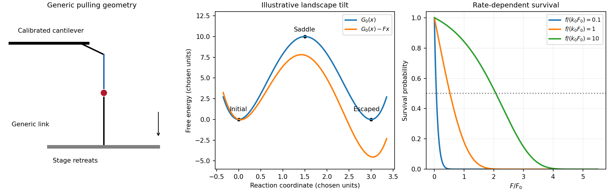
Original generic pulling arrangement, tilted energy landscape and calculated survival under a force ramp
. Details. Past exam of the soft matter and biological physics course of the University of Cambridge 2013 Paper 1 1 Solution by Codex 0 2026-10-20
Codex 0 2026-10-20For the generic instrument, magnetic tweezers combine a magnetically responsive bead, a controllable magnetic field gradient, a tether attached to a fixed support, and optical tracking of bead coordinates. For a fixed magnetic dipole moment, the force is ; an induced linear isotropic moment instead gives . A uniform magnetic field can orient an anisotropic bead, but a gradient is needed for translation. Magnet height sets the load, while field rotation can impose torque if bead orientation is coupled to the field. Tracking uses lateral images and a calibrated axial image/defocus response; a fixed reference removes stage drift. A sufficiently slowly varying gradient approximates a force clamp over the bead's displacement. TODO: user-deferred biomolecular implementation; DNA-specific attachment, preparation and response are not treated.
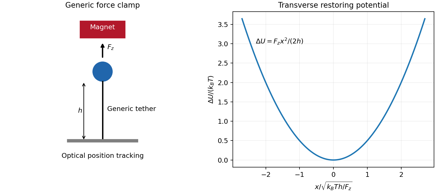
For transverse-fluctuation calibration of a tensioned tether, use an ideal tether of vertical extension whose endpoint is displaced by small . Keeping its length fixed to quadratic order lowers its vertical coordinate by , increasing load potential by . The equipartition theorem therefore givesHere fluctuations are about the mean. The height is the effective pendulum length of the measured coordinate, not automatically the polymer contour length. The displayed formula uses the point-endpoint or fixed-bead-orientation idealization; freely rotating large beads can require a bead-radius correction to that lever arm. The finite-exposure correction to fluctuation force calibration restores variance lost through exposure averaging; ignoring it would overestimate force; localization noise increases it and would underestimate force. Drift, wall coupling, finite observation time and magnetic lateral stiffness must be checked. Vertical fluctuations measure longitudinal stiffness and do not obey the same geometrical formula.
For the stretch and twist coefficients of an elastic filament, take as reference contour length and as local axial strain. The three positive quadratic costs represent bending of the tangent, stretching of the material and excess twist about its relaxed orientation. With the paper's coefficient convention, are bending and torsional rigidities with units of energy times length; is an axial force modulus. Thus have units of length and inverse length. Positive quadratic forms describe a stable relaxed filament; odd terms vanish when expansion is about its zero-stress, zero-torque reference configuration.
At weak and intermediate tension, changing thermal bending conformations can extend the filament without appreciably stretching the backbone. Axial strain is , so material stretching must be included when this is no longer negligible. For a long strongly aligned but nearly inextensible three-dimensional worm-like chain, the thermal extension deficit is approximately ; stretch adds approximately to fractional extension. Twist matters whenever torque or imposed end rotation is present, at any tension. A freely swivelling, torque-free tether need not store excess twist. There is no universal force-only threshold for switching on torsional energy.
The circular bending energy of an elastic filament follows because curvature is over contour length . Integrating the bending term givesThis is bending energy alone: imposed tension, stretching and twist would add costs. The dimensionless bending action is . Its tangent propagator in three dimensions obeys rotational diffusion on the unit sphere, . The vector spherical harmonic has angular eigenvalue , givingHence is the persistence length in this three-dimensional convention. A strictly planar filament instead has tangent-correlation length ; one cannot infer the factor merely by setting a loop's energy equal to .
TODO: user-deferred biomolecular applications. Both enzyme-driven unwinding experiments, their experimental sketches, the requested numerical force and plectoneme radius, energy loss per turn and enzyme-specific dissipation mechanisms remain unsolved. None of their biomolecular parameters has been used in a calculation.
Past exam of the soft condensed matter course of the University of Cambridge 2016 Paper 1 4 Solution by Codex 0 2026-10-20
Codex 0 2026-10-20Polydispersity means that a sample contains chains of different molar masses or lengths. Let count chains with molar mass . The number-average molar mass gives every chain equal weight, while the weight-average molar mass weights a chain population by its contribution to total mass:Writing makes the latter interpretation explicit: . Large chains therefore influence more strongly. If brackets denote an average over chain number,The ratio is molar-mass dispersity, conventionally written Đ. It equals one only when every chain has the same molar mass. Different distributions can share the same ratio, so it does not specify the full distribution.
For a freely jointed chain, write the end-to-end vector as the sum of independently oriented steps , each of fixed length . Isotropy gives , and independence gives for . HenceThe root-mean-square end-to-end distance of a polymer chain is , although the mean vector is zero. Its polymer contour length is , an upper bound on extension; it is not the typical unforced end-to-end length.
Stiffness correlates neighboring bond directions, so the discarded cross terms need not vanish. A freely rotating chain fixes the angle between successive forward bond vectors but leaves torsion uniformly distributed. Set , so . ThenFor a chain long compared with its orientational correlation range, the characteristic ratio of a freely rotating chain approaches . Positive forward persistence increases the mean-square size and gives the Kuhn length of a freely rotating chain . A chemical internal bond angle is supplementary to the forward-vector angle used here, so substituting that internal angle requires . For at fixed , the finite sum tends to , the rigid-rod result; taking the long-chain limit first would incorrectly predict an unbounded size. Real torsional energy preferences can be represented by a rotational isomeric state model, with weighted torsional states and correlations beyond independent free rotations.
A worm-like chain describes continuously varying local orientation. For unit tangent and bending stiffness , its elastic energy is . In three spatial dimensions the persistence length is andSince , integrating the tangent correlation gives the end-to-end distance of a worm-like chain:For , expansion gives , approaching a straight rod. For , it gives , the long-chain ideal chain result with Kuhn length . These models isolate stiffness; long-range excluded volume can additionally swell an isolated chain in a good solvent. When coarse-graining, a chemical repeat count and a count of independent statistical steps must not be silently interchanged.
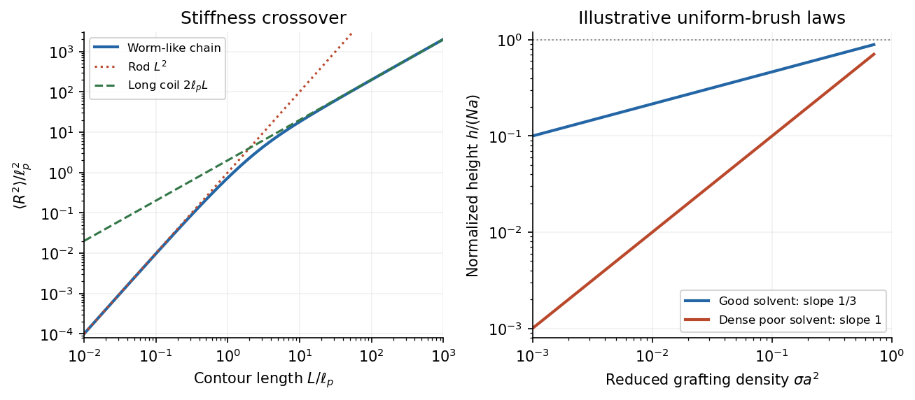
Stiff-chain crossover and distinct polymer brush density scalings
. Details. The first panel shows the exact worm-like chain crossover between a rod and a long flexible coil. The second compares original normalized scaling curves for a uniform polymer brush; their prefactors have been chosen for illustration and do not fit the exam's experimental points.
For a good solvent, consider long flexible grafted polymer chains with grafting density and lateral spacing . At high coverage, is smaller than the isolated coil size, and adjacent chains cannot retain their unperturbed conformations. A scaling model divides each chain into concentration blobs of diameter . Inside one blob the chain retains good-solvent statistics,using the Flory approximation exponent . The blobs per chain form a stretched sequence approximately normal to the surface. The good-solvent brush height therefore obeysHere and refer to consistently chosen effective segments, whose microscopic properties are held fixed as chain length changes. The result is a scaling law with an undetermined order-one prefactor, not a fully specified height in nanometres.
A complementary free-energy balance per chain iswhere is effective segment excluded volume. The first term is the chain entropy cost of stretching and the second is the cost of crowding segments into a layer of volume per chain. Minimization gives ; with it recovers the same height. The blob argument incorporates good-solvent correlations more directly. Both descriptions require overlapping chains, many segments per chain, and heights below the polymer contour length; the power law cannot be extrapolated to infinite grafting density.
In the printed experimental graph, the vertical axis is and the horizontal axis is . The approximately straight trend through the origin therefore means . Since and is proportional to chain length for a fixed repeat chemistry,The dashed guide rises by roughly – vertical units over six horizontal units, corresponding to of order per unit of the plotted . This is an approximate graphical slope, not a fitted material constant; the graph does not specify a numerical monomer count or a repeat-unit volume from which an absolute brush height could independently be calculated.
The poor-solvent brush height has a simple volume argument. Let be the volume per repeat and the roughly fixed polymer volume fraction within a dense uniform layer. There are repeats per substrate area, soFor fixed poor-solvent conditions, is approximately independent of and , giving the observed linear grafting-density dependence. Polymer–polymer contacts are favored and the layer becomes relatively compact; in a good solvent, favorable solvent contact and segment repulsion instead produce a swollen layer whose stretching and osmotic costs balance at the weaker dependence. Sparse isolated polymer globules or lateral segregation fall outside the uniform-brush model.
The cited experimental paper's abstract independently reports these two scaling laws, but identifies polydimethylsiloxane chains on porous silicon dioxide, rather than the polystyrene system named in the exam. The solution uses the printed axes to infer the exponents and does not treat that material identification as verified experimental provenance.[ref]
Characterization of the brush regime for grafted polymer layers at the solid-liquid interface by P. Auroy and others. Physical Review Letters 66 (1991), 719–722, abstract: neutron-scattering measurement, chemical system, and good- versus poor-solvent thickness scaling
Past exam of the soft condensed matter course of the University of Cambridge 2016 Paper 1 3 Solution by Codex 0 2026-10-20
Codex 0 2026-10-20A colloid has dispersed constituents whose relevant dimensions are mesoscopic: roughly to in at least one direction. Interfaces and Brownian motion are consequently important. The size range is a useful convention, not a sharp boundary separating all physical behaviour. A sol of fine silicon dioxide particles in water illustrates solid in liquid; an oil-in-water emulsion illustrates liquid in another immiscible liquid; and a foam illustrates gas dispersed in a liquid, with thin intervening films supplying the small structural dimension. A colloid need not be a thermodynamic equilibrium state.[ref]
Definition and classification of colloids by International Union of Pure and Applied Chemistry. Definition and classification of colloids: approximate size range, colloidal dispersions, sols, emulsions and foams
Unprotected particles attract through Van der Waals forces. For two equal spheres of radius with a small surface gap , the near-contact van der Waals attraction of spheres iswhere the Hamaker constant is positive for the attractive case. The large number of interacting constituent molecules can give a well much deeper than , even though individual molecular attractions are weak. Brownian motion brings particles together, and a sufficiently deep attractive well makes separation unlikely. This gives particle aggregation; solid particles can remain distinct within a cluster rather than merging into one continuous solid. Emulsion droplets can additionally coalesce if the separating film ruptures.
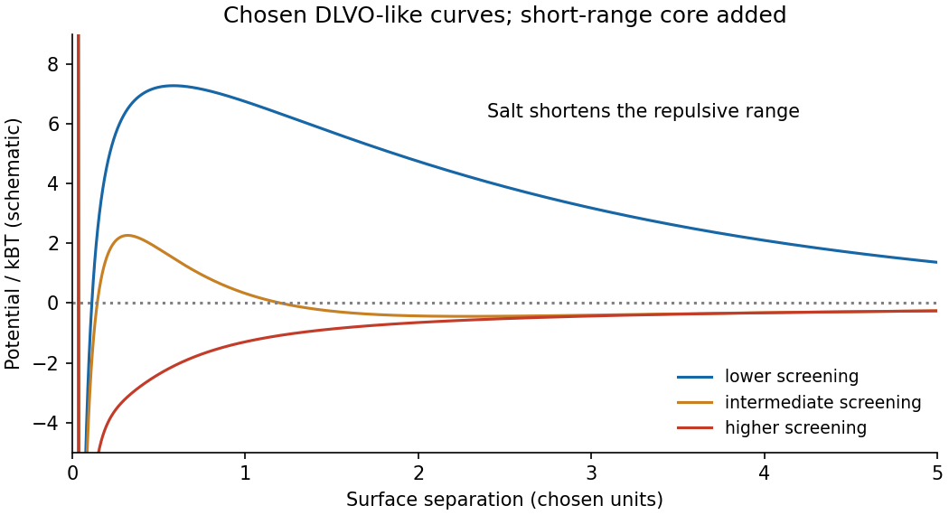
Charge stabilization of colloids supplies a repulsive barrier. Like-charged surfaces carry compensating counterions and electric double layers; bringing the layers together costs free energy. DLVO theory combines this repulsion with Van der Waals forces. A barrier large compared with can make aggregation slow, even when sticking would lower the final free energy. Adding salt generally shortens the Debye–Hückel screening length and can lower the barrier; surface charge regulation and specific ion interactions also matter. A negatively charged particle and a positively charged particle need not repel.
Steric stabilization instead coats each particle with adsorbed or grafted polymer chains. In a good solvent, overlap and compression of these layers raise the osmotic pressure and reduce chain entropy, opposing close contact. Electrosteric stabilization combines the two mechanisms. Dense, securely bound layers matter: incomplete adsorption can allow polymer bridging, while nonadsorbing dissolved polymers can create an attractive depletion force. Poor solvent quality can collapse a protective layer. Reducing the density mismatch slows sedimentation but does not remove the interparticle attraction, so uniform suspension and resistance to aggregation are different requirements.
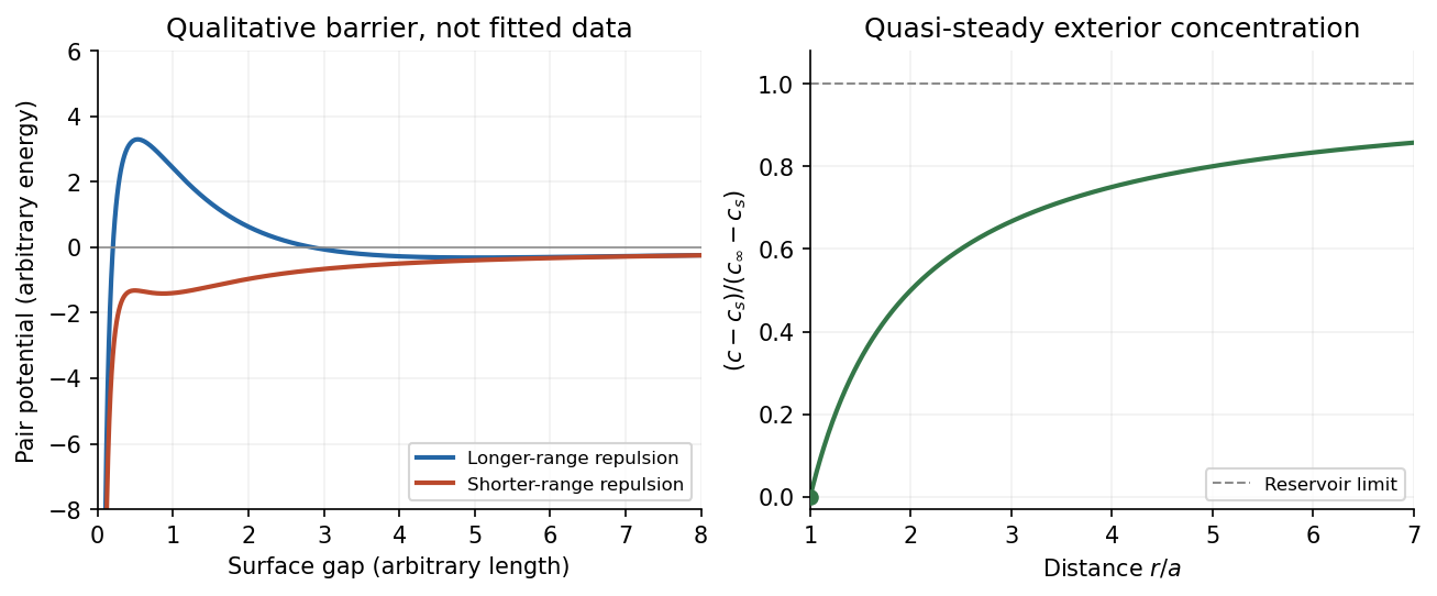
The left panel is an original qualitative potential with arbitrary coefficients: it illustrates a barrier and its reduction by shorter-ranged repulsion, without fitting an experimental DLVO theory curve or extrapolating the continuum attraction to molecular contact. The right panel plots the derived quasi-steady concentration profile in dimensionless variables.
In diffusion-controlled growth, attachment is rapid and delivery through the surrounding medium is the bottleneck. The growing surface depletes the neighboring solute, so a substantial concentration gradient develops. In reaction-controlled growth, arrival is fast compared with incorporation; many arrivals fail to attach, and the surface concentration stays near the reservoir value. The analogous distinction for particle aggregation is between near-unit sticking probability in diffusion-limited cluster aggregation and barrier-suppressed sticking in reaction-limited cluster aggregation. Here the subsequent calculation concerns accretion onto one growing particle, rather than a collision kernel for two mobile clusters.
The printed time-dependent equation is the diffusion equation, not the usual Poisson equation. For constant diffusion coefficient , no bulk sources and negligible advection, Fick's laws give the number flux . Local conservation of mass, expressed here as conservation of the accreting constituent, then givesAn arbitrary time-independent exterior profile does not solve the full moving-boundary problem exactly. The required elementary result uses a quasi-steady approximation: diffusion establishes the exterior profile much faster than the particle radius changes. At each instantaneous radius , set . Thus the exterior field solves the homogeneous Laplace equation,Two integrations give . The two boundary conditions fixFor growth, , so the profile increases outwards. Its radial flux is negative, and the positive inward arrival rate isA material density is needed to turn an arrival rate into a radial velocity. Introduce the constant constituent number density inside the particle, using the same units as . The sharp-interface balance, neglecting exterior advection, isThe difference accounts for material already present in the volume swept by the growing interface. In the usual dilute-feed approximation , it can be replaced by . With constant reservoir and surface concentrations, integration from radius gives the constant-reservoir diffusion-controlled particle growth lawConsequently when the growth contribution dominates . For a finite seed at the literal limit , the increment is instead initially proportional to . Here “early time” means before appreciable reservoir depletion or interactions with other particles, while already beyond the rapid initial establishment of the diffusion field. Indeed, the ratio of diffusion-adjustment time to radial-growth time is ; small supersaturation relative to the particle density makes the quasi-steady approximation self-consistent. No initial concentration field was specified, so an exact transient solution is not uniquely determined.
For comparison, let a finite surface-attachment coefficient be and the equilibrium surface concentration be . In the dilute-feed approximation, the Robin boundary condition givesFor this recovers transport control; for , the surface-reaction-controlled particle growth has approximately constant . Thus reaction control gives , in contrast to the diffusion-controlled square-radius law. No numerical or is supplied or needed for these scaling results.
Past exam of the soft condensed matter course of the University of Cambridge 2015 Paper 1 4 Solution by Codex 0 2026-10-20
Codex 0 2026-10-20In a regular solution, ideal combinatorial entropy competes with a nonzero unlike-contact energy. For equal molecular volumes and mole fraction of species A, write mixing free energy per site aswhereHere is the coordination number and a pair-contact energy counted consistently in the lattice model. A positive penalizes unlike contacts; a negative value favors them. The logarithmic terms lower free energy on mixing. The sign of the enthalpy of mixing alone therefore does not determine miscibility.
At fixed temperature and composition, a homogeneous phase is globally stable only if no division into two compositions lowers its free energy. The common-tangent construction selects coexisting compositions , equivalent to equality of both species' chemical potentials. Local stability to infinitesimal fluctuations instead requiresZero curvature gives the spinodal, while the coexistence boundary is the binodal. Between them a homogeneous state can be metastable and require nucleation; inside the spinodal its small composition fluctuations grow. The symmetric regular solution hasBelow this contact penalty, the free energy is convex at every composition. Above it a miscibility gap is possible around the central composition. If with , heating promotes mixing, but specific interactions or temperature-dependent noncombinatorial terms can produce other trends.
For two polymers, let count equal-volume segments per chain, and now let be the segment volume fraction of A. Connecting segments into chains reduces their independent translational entropy. The binary Flory-Huggins polymer blend hasThe energetic contact term remains extensive in the number of segments, while the favorable entropy per segment is reduced by and . This is the key long-chain limit of polymer-blend miscibility: a small positive incompatibility can overcome the mixing entropy. The lattice treatment is a controlled model for this argument, rather than a claim that every real blend has composition-independent .[ref]
Thermodynamics of High Polymer Solutions by Paul J. Flory. 1942, pp. 51–55: chain-connected lattice configurations and combinatorial mixing entropy; later sections add the energetic contribution
The local stability condition and critical interaction parameter becomeFor equal chain lengths, . Similar segment chemistry and matched cohesive interactions can reduce the unlike-contact penalty; favorable specific interactions, such as complementary hydrogen bonding, can make mixing favorable even for long chains. Lower molar mass increases mixing entropy. temperature can help when it lowers the effective , but heating is not universally sufficient. A suitable common solvent can facilitate processing or ternary mixing, and a block-copolymer compatibilizer can stabilize fine domains; neither guarantees that the final solvent-free binary material is one equilibrium molecular phase.
An oil–water emulsion illustrates emulsion stability versus molecular miscibility. A surfactant adsorbs with its water-affine head toward water and its oil-affine tail toward oil, lowering interfacial tension and the work needed to make additional interface. Breaking a fixed oil volume into spherical droplets of radius gives total area , so creating small droplets still requires substantial area and usually mechanical work.
Adsorbed surfactants can oppose droplet coalescence through charged double-layer repulsion, hydrated-head interactions or steric repulsion from sufficiently extended groups. Adequate coverage, adsorption time, ionic conditions and film drainage affect the lifetime. A lower interfacial tension does not itself remove the bulk miscibility gap, and a protected emulsion is commonly kinetically stabilized. A thermodynamically stable microemulsion is a distinct situation requiring an appropriate composition and free-energy balance. The two liquids must not be called molecularly miscible simply because droplets disperse visibly.
For the capillary, balance upward contact-line force against hydrostatic column weight, neglecting meniscus volume and gas density. For inner radius ,The contact angle is measured through the liquid. complete wetting means , so the contact-angle change of capillary rise givesThis follows from the stipulated wetting change, holding radius, bulk liquid surface tension and density fixed. One should not replace that premise with a general claim that grease always improves glass wetting; if contamination also changes the liquid surface tension, the original height and new angle alone would not determine the new height.
For two wide vertical plates separated by gap , use unit width. There are two upward contact-line contributions and liquid cross-sectional area , giving the capillary rise between parallel plates:Only one principal meniscus curvature contributes between wide plates, whereas a circular tube has two. For the same fluid and angle,If the plate gap equals the tube diameter, , the rise is half as large: the initial and completely wetting heights would be cm and cm. If instead , the heights are equal. In either geometry, changing only the angle from to zero multiplies the height by . Since the question specifies no plate spacing, the general gap-dependent relation is the unambiguous result; the half-height answer requires the equal-gap-to-diameter convention.
Past exam of the soft condensed matter course of the University of Cambridge 2015 Paper 1 3 Solution by Codex 0 2026-10-20
Codex 0 2026-10-20An amphiphile has a solvent-affine part and a solvent-averse part within one molecule. In water these are commonly called hydrophilic head and hydrophobic tail. Two nonbiological examples are sodium dodecyl sulfate, with a twelve-carbon tail and an anionic sulfate head, and cetyltrimethylammonium bromide, with a sixteen-carbon tail and a cationic quaternary-ammonium head. Their counterions balance the ionic head-group charge; the head and tail do not have interchangeable interactions with water.
Aggregation reduces unfavorable exposure of hydrocarbon tails to water but loses molecular translational entropy. Interfacial free energy, head-group solvation and electrostatic repulsion, chain packing and conformational entropy determine the preferred aggregate. The hydrophobic effect is a solvent-mediated free-energy balance, rather than a literal attractive bond between tails.
The amphiphile packing parametercompares tail volume , effective head-group area and maximum tail length . A spherical core of radius obeys , and a long cylindrical core obeys . The condition gives the conventional spherical window and cylindrical window . Less strongly curved bilayers become compatible for , with planar packing near one; values above one can favor inverse curvature in an appropriate nonpolar surrounding medium. These windows are geometric guides rather than exact phase boundaries.
A larger hydrated or electrostatically repelling head increases and favors positive curvature. Screening of charged heads or a smaller head can lower and favor rods or sheets. Multiple tails increase the tail volume relative to head area and can favor bilayers. Tail length, branching, temperature and solvent selectivity alter both geometry and interaction free energy, so one cannot predict a unique aggregate from hydrophobicity alone.[ref]
Theory of self-assembly of hydrocarbon amphiphiles by Jacob N. Israelachvili and others. 1976, pp. 1525–1568: coupled thermodynamics, molecular packing constraints and globular, cylindrical and bilayer aggregates
In the supplied chemical-potential expression, is the equilibrium chemical potential per amphiphile, the standard free energy per amphiphile within an aggregate of size , and the dimensionless molecular fraction belonging to that size class. The aggregate molecular fraction versus aggregate number fraction distinction explains the logarithm: the aggregate count fraction is , and dividing its translational chemical potential by gives a per-molecule value. ThusHere is the Boltzmann constant, absolute temperature, and a positive integer. The logarithm acts on a dimensionless ideal activity; a concentrated nonideal solution would require activity coefficients.
equilibrium exchange of amphiphiles gives the same per-molecule for every size. For monomers, . Substitution yields the finite-micelle aggregation-number distributionThis formula by itself does not prescribe a preferred micelle size: the size dependence of must include the competing packing and interaction terms. If their balance favors a finite size , a monomer population and a peak around that size can coexist. Dividing by would instead plot the distribution of aggregate counts.
At very low , the factors suppress large aggregates and most molecules remain monomers. As rises, a favorable aggregate class grows extremely rapidly because of this high power. The critical micelle concentration from standard chemical potentials has the large-size estimateMore precisely, the illustrative crossover condition givesAdded material above the crossover enters aggregates predominantly. Monomer concentration then increases slowly rather than being exactly pinned: its logarithm enters , while aggregate populations respond with a large factor . For finite micelles this is a sharp association crossover, not an absolute prohibition on aggregates below one exact concentration.
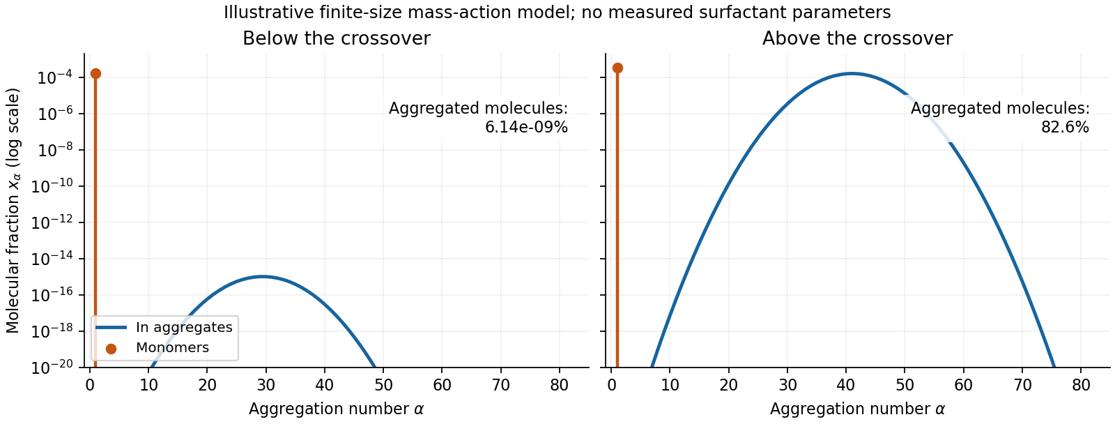
Original illustrative molecular-fraction distributions over aggregation number below and above a micellization crossover
. Details. The drawing uses a declared illustrative standard-free-energy model favoring aggregates near . It is not an inferred distribution or critical concentration for either named surfactant. The separate monomer peak is at ; a distribution of molecular fractions weights each aggregate by its number of molecules.
For the general physics of a nearly planar fluid sheet, let be a small-slope displacement, membrane bending rigidity and mechanical tension. At fixed topology and symmetric reference curvature, the quadratic Helfrich energy isThe bending term is the small-slope curvature-elastic energy; additional spontaneous-curvature or boundary terms require extra information.[ref]
Elastic Properties of Lipid Bilayers: Theory and Possible Experiments by Wolfgang Helfrich. Section II.C, p. 695, equation (12): curvature-elastic energy and coefficients with units of energy
For Fourier amplitudes , equipartition gives the membrane fluctuation spectrum under tension,Higher temperature increases fluctuations, while greater membrane bending rigidity or tension suppresses them. Short-wavelength modes are predominantly bending-controlled; longer wavelengths can be tension-controlled. Finite sheet size, supports, confinement and imposed area set boundary conditions and infrared cutoffs; continuum elasticity also needs a short-distance cutoff. solvent viscosity affects relaxation rates, although it does not enter this equilibrium amplitude at fixed elastic parameters.
TODO: user-deferred biology. The requested importance of these fluctuations for bodily function is deferred. The preceding result covers only the independent continuum and thermal physics.
Past exam of the soft condensed matter course of the University of Cambridge 2014 Paper 1 4 Solution by Codex 0 2026-10-20
Codex 0 2026-10-20Balancing buoyant weight with Stokes drag givesThis needs isolated spherical particles, low Reynolds number and negligible wall corrections. The supplied settling measurement gives , hence . Its Reynolds number is about , consistent with the approximation.
Compare gravitational work over one radius with thermal energy, or use with . The gravitational Peclet number givesBelow this sedimentation-Brownian crossover radius Brownian motion dominates settling on the particle-size scale. It does not eliminate gravity: the sedimentation scale height is . For negligible concentration gradients across a sample height , the stronger condition is . No universal permanently nonsedimenting size follows without a length/time criterion.
Brownian encounters bring small particles into contact; van der Waals attraction can then bind them. Surface charge can create a repulsive barrier through Debye screening of colloid repulsion. For a monovalent salt reservoir with number density of each ionic species, Poisson–Boltzmann theory hasFor , linearization gives , with . If instead means total ion density, the factor two is absent. The planar potential decays as ; a sphere has an additional factor. This mean-field approximation neglects specific adsorption, ion correlations and finite ion size.
DLVO theory adds screened repulsion to dispersion attraction. At small surface separation for equal spheres of radius , a useful schematic form iswith a short-range repulsive core needed outside the continuum model. Low salt can leave a barrier many times , giving kinetic stability. Higher salt shortens the repulsion and can lower or remove the barrier, allowing coagulation into a deep primary minimum. The primary and secondary DLVO minima have different consequences: a shallow secondary minimum permits looser, sometimes reversible aggregation. The surface boundary condition affects ; screening length alone is not a complete measured interaction law. Non-DLVO hydration or steric forces can matter at contact.
Pinned article: Introduction to the OurBigBook Project
Welcome to the OurBigBook Project! Our goal is to create the perfect publishing platform for STEM subjects, and get university-level students to write the best free STEM tutorials ever.
Everyone is welcome to create an account and play with the site: ourbigbook.com/go/register. We belive that students themselves can write amazing tutorials, but teachers are welcome too. You can write about anything you want, it doesn't have to be STEM or even educational. Silly test content is very welcome and you won't be penalized in any way. Just keep it legal!
Intro to OurBigBook
. Source. We have two killer features:
- topics: topics group articles by different users with the same title, e.g. here is the topic for the "Fundamental Theorem of Calculus" ourbigbook.com/go/topic/fundamental-theorem-of-calculusArticles of different users are sorted by upvote within each article page. This feature is a bit like:
- a Wikipedia where each user can have their own version of each article
- a Q&A website like Stack Overflow, where multiple people can give their views on a given topic, and the best ones are sorted by upvote. Except you don't need to wait for someone to ask first, and any topic goes, no matter how narrow or broad
This feature makes it possible for readers to find better explanations of any topic created by other writers. And it allows writers to create an explanation in a place that readers might actually find it.
Figure 1. Screenshot of the "Derivative" topic page. View it live at: ourbigbook.com/go/topic/derivativeVideo 2. OurBigBook Web topics demo. Source. - local editing: you can store all your personal knowledge base content locally in a plaintext markup format that can be edited locally and published either:This way you can be sure that even if OurBigBook.com were to go down one day (which we have no plans to do as it is quite cheap to host!), your content will still be perfectly readable as a static site.
- to OurBigBook.com to get awesome multi-user features like topics and likes
- as HTML files to a static website, which you can host yourself for free on many external providers like GitHub Pages, and remain in full control

Figure 2. You can publish local OurBigBook lightweight markup files to either OurBigBook.com or as a static website.
Figure 3. Visual Studio Code extension installation.
Figure 5. . You can also edit articles on the Web editor without installing anything locally. Video 3. Edit locally and publish demo. Source. This shows editing OurBigBook Markup and publishing it using the Visual Studio Code extension. 
- Infinitely deep tables of contents:




All our software is open source and hosted at: github.com/ourbigbook/ourbigbook
Further documentation can be found at: docs.ourbigbook.com
Feel free to reach our to us for any help or suggestions: docs.ourbigbook.com/#contact