Topics (384k) Articles (398k) Users (410) Discussions (242) Comments (383) Files (13k) New article
Past exam of the systems biology course of the University of Cambridge 2024 Paper 3 1 g Solution by  Codex 0 2026-10-20
The interaction term estimates that the weight-associated change in mean testosterone concentration is per gram greater in males than females: the female slope is and the male slope is per gram.
Past exam of the systems biology course of the University of Cambridge 2024 Paper 3 1 f Solution by Codex 0 2026-10-20
Codex 0 2026-10-20Include both main effects and their interaction term:
fit_interaction <- lm(testosterone ~ weight * sex, data = mice)Here
mice denotes the data frame containing the named variables. In this R formula, weight * sex expands to weight + sex + weight:sex; it does not omit the main effects. Past exam of the systems biology course of the University of Cambridge 2024 Paper 3 1 e Solution by Codex 0 2026-10-20
Codex 0 2026-10-20Two assumptions of the usual normal linear model used for the reported coefficient Student t-tests are:
- The errors are independent random variables across mice.
- Conditional on the predictors, each error has a normal distribution with mean zero and the same variance : .
The second statement includes homoscedasticity. Normality concerns the conditional errors, rather than requiring the weights themselves to have a normal distribution.
Past exam of the systems biology course of the University of Cambridge 2024 Paper 3 1 d Solution by Codex 0 2026-10-20
Codex 0 2026-10-20At a conventional 5% significance level, there is evidence for an association with sex after adjusting for weight, because its two-sided p-value is . There is insufficient evidence for a weight association after adjusting for sex, because its p-value is .
These Student t-tests test whether the corresponding regression coefficients are zero within the additive multiple linear regression. Failure to reject the weight hypothesis does not establish an exactly zero effect; these associations alone also do not justify a causal inference. The later model with a statistical interaction asks a different question, allowing the weight association to differ by sex.
Past exam of the systems biology course of the University of Cambridge 2024 Paper 3 1 c Solution by Codex 0 2026-10-20
Codex 0 2026-10-20At the same weight, male mice have an estimated mean testosterone concentration higher than female mice; the sex regression coefficient is an adjusted difference between the groups.
Past exam of the systems biology course of the University of Cambridge 2024 Paper 3 1 b Solution by Codex 0 2026-10-20
Codex 0 2026-10-20Holding sex fixed, each additional gram of weight is associated with an estimated increase in mean testosterone concentration, according to the fitted multiple linear regression.
Past exam of the systems biology course of the University of Cambridge 2024 Paper 3 1 a Solution by Codex 0 2026-10-20
Codex 0 2026-10-20The estimated intercept means that a female mouse with weight zero would have predicted mean testosterone concentration under this linear regression; zero weight is an extrapolation without a meaningful adult-mouse interpretation.
Past exam of the systems biology course of the University of Cambridge 2024 Paper 2 6 iv Solution by Codex 0 2026-10-20
Codex 0 2026-10-20Stochastic optical reconstruction microscopy separates emitters in time rather than shrinking every illuminating spot. Switch only a sparse subset of labeled molecules into a fluorescent state, localize their individual point spread functions, switch or bleach them off, and repeat. Combining many fitted positions reconstructs structure finer than the individual diffraction-blurred spots.[ref]
Sub-diffraction-limit imaging by stochastic optical reconstruction microscopy (STORM) by Michael J. Rust and others. pp. 793–795, sparse activation and localization reconstruction
An interesting application is the neuronal axon. STORM revealed approximately – periodic organization of actin, spectrin and associated proteins, supporting a membrane-associated cytoskeletal architecture that ordinary fluorescence images did not resolve clearly.[ref]
Localization precision improves with detected photons, but reconstructed resolution also depends on label density, label size, drift and reliable separation of emitters. Many frames are needed, so motion and slow acquisition can limit live imaging. Multiple localizations of one blinking label must not automatically be counted as multiple molecules. A precise molecular fit and a faithful reconstructed biological structure are related but distinct achievements.
Past exam of the systems biology course of the University of Cambridge 2024 Paper 2 6 iii Solution by Codex 0 2026-10-20
Codex 0 2026-10-20Stimulated emission depletion microscopy narrows the region allowed to emit detectable fluorescence. A focused excitation pulse or beam populates the excited state. A red-shifted depletion beam with a central intensity minimum drives stimulated emission from the surrounding excited fluorophores. The stimulated photons are rejected from the fluorescence detection channel, leaving spontaneous emission concentrated near the depletion zero. Scanning this small effective emission region builds the image.[ref]
Breaking the diffraction resolution limit by stimulated emission: stimulated-emission-depletion fluorescence microscopy by Stefan W. Hell and others. pp. 780–782, depletion of the outer excitation region and proposed beam geometry
Near an ideal zero, take depletion intensity proportional to squared radius. The radius at which it reaches a saturation scale decreases as the depletion amplitude grows. A common approximate resolution law iswhere is the undepleted characteristic width and depends on fluorophore kinetics and illumination timing. It is an idealized scaling, not a universal instrument calibration. For example, a threefold width reduction needs in this model. The illumination beams remain diffraction limited; nonlinear control of the emitting population creates the smaller effective response.
The cost is high depletion intensity, with possible photobleaching, phototoxicity and heating, demanding fluorophore photophysics, precise beam alignment and maintenance of the central zero. Point scanning limits speed and trades off field size, dwell time and photon statistics. Scattering and aberrations can fill the depletion minimum and degrade performance in depth. A simple lateral doughnut mainly improves lateral resolution; improved axial confinement requires an appropriate three-dimensional depletion pattern. Resolution gain is therefore conditional on usable photons, sample integrity and the actual depletion geometry.
Past exam of the systems biology course of the University of Cambridge 2024 Paper 2 6 ii Solution by Codex 0 2026-10-20
Codex 0 2026-10-20Start with the biological quantity to measure: compartment location, molecular colocalization, fast cell dynamics, deep-tissue activity or nanometre-scale organization. Specify the required field, depth, lateral and axial resolution, temporal sampling and acceptable perturbation before choosing the instrument.
For a thin fixed specimen or a shallow live preparation, confocal microscopy provides flexible multicolour imaging and effective optical sectioning with widely available labels. Adjust the pinhole and dwell time against signal-to-noise ratio, bleaching and speed. Repeatedly scanning a large volume can become too slow, and out-of-focus excitation can damage regions that contribute little useful signal.
For a living scattering specimen, two-photon excitation microscopy often offers better access to depth and confinement of excitation. Longer excitation wavelengths scatter less strongly in many tissues, and broad collection can recover scattered emission without a detection pinhole. These benefits do not eliminate depth-dependent optical aberrations, absorption, heating or focal phototoxicity. Pulsed excitation can also make instrumentation and suitable multicolour excitation more demanding.
If the priority is rapid, gentle volumetric observation of a suitable specimen, consider light-sheet fluorescence microscopy rather than forcing either point-scanning method to cover every use case. If subdiffraction molecular organization is required, consider a suitable super-resolution method and assess its labeling, speed and dose costs.
Finally, calibrate the point spread function in a sample-relevant medium, sample finely enough in all three dimensions, and check registration between colour channels. Match photon collection and exposure to the question, with controls for label-induced changes and photobleaching. The best method meets the biological resolution and timing requirements with sufficient signal and acceptable perturbation; the smallest nominal resolution number alone does not decide.
Past exam of the systems biology course of the University of Cambridge 2024 Paper 2 6 i Solution by Codex 0 2026-10-20
Codex 0 2026-10-20 The compact emitting region in (a) indicates that excitation itself is strongly localized. In (b), the illuminated path generates out-of-focus fluorescence as well as fluorescence near the focus. A confocal detection pinhole can reject much of that unwanted emission from the recorded image; it does not prevent the dye solution from emitting it.
In ordinary one-photon excitation, the local fluorescence-generation rate is approximately proportional to excitation light intensity . In unsaturated two-photon excitation microscopy, it is proportional to . Simultaneous absorption is appreciable only in the high-intensity focal region, generally produced using a pulsed laser. Two lower-energy photons jointly excite the fluorophore; the excitation wavelength is therefore typically substantially longer than in its one-photon experiment. This reduces out-of-focus excitation and permits detection without a confocal pinhole.[ref]
Two-photon laser scanning fluorescence microscopy by Winfried Denk and others. pp. 73–75, quadratic excitation, optical sectioning and pulsed illumination
For a small detection pinhole, the effective confocal point spread function is approximatelyHere each factor denotes an intensity response. Excitation and detection jointly select the focal region. Enlarging the pinhole increases collected signal but weakens axial rejection and changes the effective point spread function. In two-photon excitation microscopy with broad collection, the spatial response is dominated byThe pinhole product and excitation square are different physical mechanisms even when simplified mathematical profiles resemble one another.[ref]
Confocal microscopy (chapter manuscript) by Brad Amos and others. Confocal formation and conjugate focal selection, Fig. 3; discussion of excitation and detection responses
Compare both lateral and axial widths using the actual wavelengths and objective. For a diffraction-limited system, their characteristic scalings arewhere is numerical aperture and is the medium's refractive index. Numerical prefactors depend on the width criterion and high-aperture optical model. Axial resolution is generally worse than lateral resolution. A small confocal pinhole improves axial sectioning and can narrow the lateral response, at the cost of photon throughput.
As a simple Gaussian function example, has squared profile , so its width is reduced by . However, the two-photon illumination spot itself is broader at its longer excitation wavelength. Two-photon excitation is not automatically higher-resolution than confocal microscopy, and ordinary two-photon sectioning is not intrinsically super-resolution. Compare measured point spread functions, pinhole settings, numerical apertures, scattering and optical aberrations, not just the fact that one profile is squared.
The original model figure below separates focal confinement from wavelength-dependent width. It is an illustrative one-dimensional Gaussian function calculation, not a reproduction or quantitative fit of the supplied photograph.
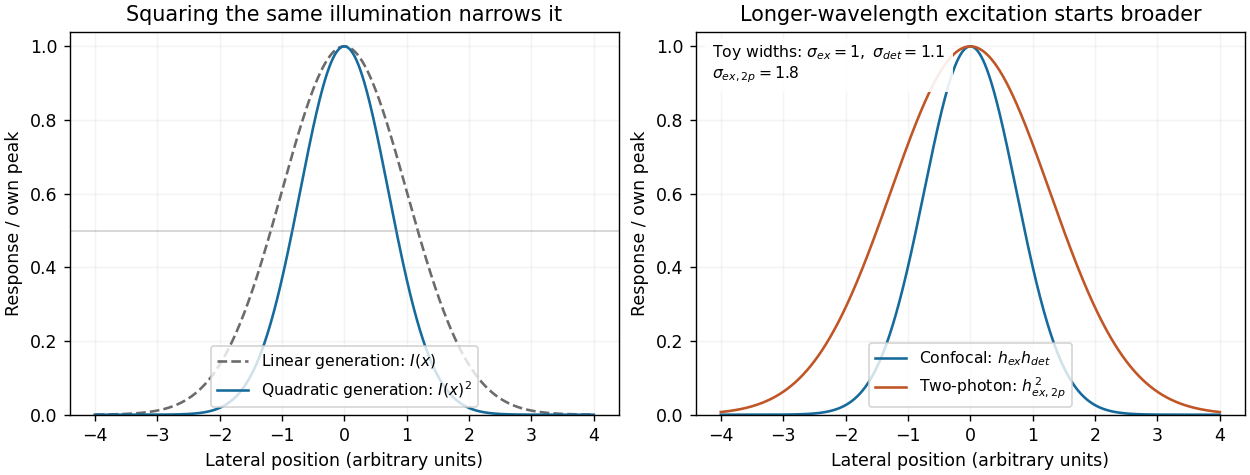
Local excitation nonlinearity and wavelength-dependent point-spread widths
. Left: squaring the same normalized Gaussian illumination narrows the local generation profile. Right: a longer-wavelength illumination profile can remain broader after squaring than an illustrative confocal excitation-times-detection response. All widths are synthetic; peak normalization does not equate photon throughput or excitation dose. Details. Past exam of the systems biology course of the University of Cambridge 2024 Paper 2 3 ii Solution by Codex 0 2026-10-20
Codex 0 2026-10-20Structural analysis should ask more than whether a candidate was recovered: which surfaces are near one another, which regions change on association, and how are subunits arranged? Enrichment from part (i) supplies material and candidates, but structural measurements require their own controls.
In chemical cross-linking mass spectrometry, react the assembly with a cross-linker of known chemical specificity and spacer properties, digest it and identify linked peptide pairs by tandem mass spectrometry. An inter-protein link places two reactive residues near one another in at least a sampled conformation; intra-protein links constrain folding or conformation. These constraints can test a structural model or place subunits within an assembly. The useful distance bound includes side chains and linker reach, not only the nominal spacer length. Search-space expansion and ambiguous assignments require error control at the linked-pair level, rather than borrowing an ordinary single-peptide error estimate.
In hydrogen-deuterium exchange mass spectrometry, compare the incorporation of deuterium into exchangeable backbone positions in free and bound samples over a time course. After quenching and peptide analysis, reduced exchange can reveal protected or stabilized regions. Protection may indicate an interface, but it can also arise from an allosteric change, altered hydrogen bonds or reduced structural opening. It therefore constrains a hypothesis rather than identifying a unique atomic contact.
Native mass spectrometry can examine intact assemblies and subcomplexes, providing evidence about composition and stoichiometry. Gas-phase loss and differing ionization efficiencies must be considered. Cryo-electron microscopy can then reveal overall architecture and, with sufficient data quality and suitable particle behaviour, high-resolution interfaces. Heterogeneity, flexible regions and purification artefacts can limit the reconstruction. Combining these observations is often more informative than demanding that one technique answer every structural question.
Quantitative proteomics is necessary in both enrichment and structural comparisons. For an assembled versus disrupted complex, measure component abundances as well as cross-linked-peptide signals. A decreased inter-protein link may reflect loss of one subunit rather than movement of an interface. Comparing cross-link abundance after accounting for recovered protein amounts helps distinguish these explanations. Matched labeling chemistry, reaction time, independent reactions and a dose series reduce artefacts caused by unequal cross-linking or excessive stabilization.
For hydrogen-deuterium exchange mass spectrometry, compare matched peptide sequences at multiple labeling times, control back-exchange and retain replicate uncertainty. A consistent local change without a corresponding abundance loss supports a structural effect. Differential peptide intensities, exchange measurements and the affinity-enrichment data should be interpreted together; an ordinary protein abundance ratio does not itself measure a distance or a direct interface.
Finally, test a predicted interface by changing selected residues while retaining folding and expression, then repeat the quantitative association assay. Loss of the candidate association with preserved bait integrity strengthens the interface interpretation. The convincing result connects selective recovery, structural constraints and a controlled perturbation, rather than treating one recovered band or one protected segment as a complete structure.
Past exam of the systems biology course of the University of Cambridge 2024 Paper 2 3 i Solution by Codex 0 2026-10-20
Codex 0 2026-10-20Affinity purification and proximity labeling answer related but different questions. The former enriches material that remains associated during extraction; the latter marks a neighbourhood before extraction. Neither alone proves a direct protein-protein interaction.
In affinity purification-mass spectrometry, isolate a bait protein with an antibody or an endogenous epitope tag. Lyse under conditions chosen to preserve the relevant protein complex, capture the bait on an affinity matrix, wash away background and identify co-purifying proteins by liquid chromatography-mass spectrometry after digestion into peptides. Co-immunoprecipitation is the antibody-based version of this association test. Gentle conditions preserve more weak interactions but also increase background; stringent washing improves specificity at the cost of labile partners. Extraction can disrupt membrane assemblies or create associations that were not present in intact cells.
Controls should include matched tag-only or untagged cells, an appropriate antibody control, input abundance and, where feasible, a binding-defective bait that retains its normal localization. Check that tagging has not changed the bait's abundance, localization or function. Reciprocal capture of a candidate partner is useful validation. If an association might be bridged by RNA or DNA, compare nuclease-treated and untreated samples while recognizing that nuclease treatment may dismantle a biologically genuine assembly.
For proximity labeling, fuse the bait to TurboID, which activates biotin and covalently labels accessible nearby proteins in living cells. After a timed labeling pulse, harsh lysis can be used because recovery no longer requires the original assembly to survive. Capture biotinylated material using streptavidin and identify enriched proteins by mass spectrometry. This can recover transient or insoluble neighbourhoods missed by ordinary extraction. A localization-matched control enzyme, no-added-biotin condition and matched expression help separate the bait's neighbourhood from diffuse labeling and endogenous biotinylated proteins.[ref]
Efficient proximity labeling in living cells and organisms with TurboID by Tess C. Branon and others. Figs. 1–3, enzyme activity, labeling time and compartment-specific comparisons
The label records proximity, accessibility and time spent nearby. A neighbour need not bind the bait; a real binder might label poorly if reactive groups are inaccessible. Pulse duration therefore trades temporal selectivity against labeling yield, rather than defining an exact universal distance cutoff.
Quantification distinguishes enrichment from a list of contaminants. Use label-free quantification of peptide signals across independent bait and control purifications, or SILAC in compatible cell cultures to compare light and heavy samples. In SILAC, isotope-containing amino acids enter newly synthesized proteins; matched peptides form distinguishable mass pairs. A label swap helps identify isotope-condition confounding. Tandem mass tags offer multiplexed comparison using reporter signals, but interfering co-isolated peptides can compress ratios.
Estimate enrichment and its reproducibility relative to matched controls, accounting for bait recovery and input abundance. Common abundant contaminants should not be promoted solely because many spectra identify them. Statistical scoring such as SAINT models the contrast between specific and background recovery across controls and replicates, allowing candidate associations to be ranked with estimated error rates.[ref]
SAINT: probabilistic scoring of affinity purification-mass spectrometry data by Hyungwon Choi and others. Statistical model, control purifications and interaction-probability estimation
A reproducibly enriched candidate is evidence for the assay-defined association or neighbourhood, not automatically a direct binding partner or fixed stoichiometric subunit. Past exam of the systems biology course of the University of Cambridge 2024 Paper 2 2 iv Solution by Codex 0 2026-10-20
Codex 0 2026-10-20The distinction is principally molecular readout by sequencing versus molecular readout by imaging; it does not impose one universal ranking of sensitivity or spatial resolution.
| Issue | Sequencing-based spatial transcriptomics | Imaging-based spatial transcriptomics |
|---|---|---|
| Target breadth | Many capture assays survey broad polyadenylated RNA without a fixed gene panel. | Probe-based assays usually require a designed target set, though seqFISH+ and MERFISH can be highly multiplexed. |
| Spatial information | Positions are capture features or beads; some collect mixtures of cells. | Individual molecular coordinates and subcellular distributions can be retained. |
| Sensitivity and bias | Capture, reverse transcription and library sampling lose molecules; amplification and diffusion add bias. | Probe accessibility, optical crowding, autofluorescence and decoding errors determine detection. |
| Resources | Requires sequencing capacity and barcode-aware analysis. | Requires extensive imaging, repeated fluidics, registration and image storage. |
| Cell assignment | Mixed features may need statistical estimation using reference cell profiles. | Usually needs explicit cell segmentation, which can misassign otherwise well-localized molecules. |
For discovery of unexpected gene expression programmes across a large section, broad sequencing-based capture is attractive. To test where selected transcripts lie within cells or precisely map a known anatomical niche, molecular imaging is attractive. Neither implies that every transcript is measured, and a nominal spot size should not be confused with biological assignment accuracy.
A productive study can combine broad discovery with targeted spatial validation on independent sections. Compare effective detection, tissue area, resolution, cost and replicate count for the specific implementations available, rather than treating all sequencing assays as coarse and all imaging assays as low-plex. Cells or capture spots from one donor are not substitutes for independent biological replicates.
Past exam of the systems biology course of the University of Cambridge 2024 Paper 2 2 iii Solution by Codex 0 2026-10-20
Codex 0 2026-10-20Imaging methods identify RNA molecules where they remain in the fixed specimen, rather than recovering their position through a sequencing-library address. Their common foundation is sequence-specific oligonucleotide probe binding and repeated fluorescence microscopy.
In single-molecule fluorescence in situ hybridization, many short complementary probes bind one transcript. Their combined fluorescence produces a detectable spot that can be localized and counted. Multiple probes make an individual bound molecule distinguishable from isolated-probe background. Conventional colour channels limit how many transcript species can be distinguished in one image, and overlapping spots make abundant targets difficult to count.
MERFISH. Encoding probes bind each target RNA and expose selected readout sequences. Across successive hybridization and imaging rounds, fluorescent readout probes interrogate those sequences, producing an on/off code at each molecular position. The code identifies the transcript. The codebook is designed with separation between valid words so that some missing or spurious signals can be detected and, for suitable codes, corrected. Fiducials and image registration keep the same molecule aligned across rounds. This multiplexes many targets without needing one physically separate fluorescence colour for each gene.[ref]
Spatially resolved, highly multiplexed RNA profiling in single cells by Kok Hao Chen and others. Results, encoding scheme and error-robust barcodes; Figs. 1–3
seqFISH and seqFISH+. Successive probe hybridization rounds encode a transcript through a sequence of detected colours. The expanded seqFISH+ strategy distributes targets among many pseudocolour states, so each round contains only a sparse subset of the total signals. This reduces optical crowding and makes a much larger target set readable on an ordinary confocal microscope. The original seqFISH+ study profiled about 10,000 genes in mouse brain tissue and examined both cellular organization and subcellular expression patterns.[ref]
Transcriptome-scale super-resolved imaging in tissues by RNA seqFISH+ by Chee-Huat Linus Eng and others. Abstract; Figs. 1–4, pseudocolours, optical crowding and tissue organization
These are two distinct multiplexing implementations, although both build on repeated in situ probe readout. Their performance depends on probe specificity, the codebook, stripping or inactivation of previous signals, retention of RNA, registration across rounds and the density of simultaneously visible spots. Imaging many rounds can be slow, and tissue autofluorescence or poor probe penetration can obscure molecules.
Finally, use nuclear and membrane information for cell segmentation, with checks for errors at touching cells and tissue boundaries. A precise molecular coordinate does not guarantee correct cell assignment. Negative or unused codes and independent probes help estimate false calls; biological replicates establish whether a spatial pattern is reproducible.
Past exam of the systems biology course of the University of Cambridge 2024 Paper 2 2 ii Solution by Codex 0 2026-10-20
Codex 0 2026-10-20The central principle is to attach a recoverable spatial address to an RNA-derived molecule before the tissue's positional organization is destroyed. After sequencing, each read identifies both a transcript and a capture location.
In the original array-based spatial transcriptomics method, a thin tissue section is placed on a slide carrying spatially indexed capture primers. The tissue is imaged for histology, then permeabilized. Polyadenylated messenger RNA binds the oligo(dT) region of the primers and is copied by reverse transcription. The resulting cDNA carries the positional barcode. Sequencing identifies the expressed gene, and a barcode lookup places its counts back on the tissue image. The first published array used approximately capture features, so a feature could contain contributions from several cells; it was not a single-cell measurement by construction.[ref]
Visualization and analysis of gene expression in tissue sections by spatial transcriptomics by Patrik L. Ståhl and others. pp. 78–80, spatially localized cDNA synthesis, positional barcodes and array features
Slide-seq applies the same addressing idea using a dense monolayer of roughly barcoded beads. The bead barcode–position map is decoded in advance. A tissue section is transferred onto the beads, released RNA is captured, and the sequenced molecular addresses recover the bead-level expression map. This gives much finer spatial sampling than the original coarse array, although RNA capture efficiency and assignment to individual cells remain limiting.[ref]
Slide-seq: A scalable technology for measuring genome-wide expression at high spatial resolution by Samuel G. Rodriques and others. pp. 1463–1465, bead puck construction, positional decoding and RNA capture
Some assays also incorporate a unique molecular identifier so that amplified reads from one captured molecule can be collapsed, reducing polymerase chain reaction duplication bias. Spatial barcodes identify capture locations; unique molecular identifiers identify molecules within those locations. Neither alone supplies cell boundaries.
For either method, align the coordinate map with histology, account for capture efficiency and background, and use independent tissue specimens as biological replicates. A smaller capture feature improves sampling granularity but does not guarantee equal effective spatial resolution or a pure single-cell transcriptome: tissue thickness, diffusion and mixed cell boundaries still matter.
Past exam of the systems biology course of the University of Cambridge 2024 Paper 2 2 i Solution by Codex 0 2026-10-20
Codex 0 2026-10-20Bulk RNA sequencing mixes the gene expression of all sampled cells, while dissociated-cell measurements retain individual profiles but usually lose their original neighbours and positions. Spatial transcriptomics preserves those relationships. The same cell type can behave differently at a tissue boundary, near a blood vessel or beside a tumour, so position can explain a state that a cell-type label alone cannot.
Spatial measurements can reveal tissue layers, developmental boundaries, tumour–immune interfaces and subcellular RNA localization. They can distinguish a change in cell abundance from a change in expression within a particular anatomical niche. Dissociation can also lose fragile cells or induce stress responses.
Past exam of the systems biology course of the University of Cambridge 2024 Paper 1 Section II 2.3 Solution by Codex 0 2026-10-20
Codex 0 2026-10-20A predictively useful simulation of a simple multicellular organism is a plausible long-term goal, but “fully” must specify resolution, environmental conditions and the predictions to be tested. A model that reproduces selected behaviors is attainable in a different sense from an exact simulation of every molecule throughout development, physiology, reproduction and aging. The former can be evaluated scientifically; the latter is neither established by present models nor a necessary definition of success.
A useful target might be a specified developmental stage of Caenorhabditis elegans, in a controlled environment, with predictions for cell states, body movement and responses to defined perturbations. Its small size, optical accessibility and extensively mapped cell lineage make it attractive. The classic embryonic lineage study traced divisions, cell deaths and fates, while also using perturbations to investigate the role of interactions.[ref]
The embryonic cell lineage of the nematode Caenorhabditis elegans by John Sulston and others. Abstract and cell-ablation experiments, lineage description versus developmental mechanism
Such a map constrains what a simulator must reproduce, but a list of normal outcomes does not itself specify the rules that generate them or how those rules respond to an unfamiliar intervention.whole-cell modeling demonstrates both progress and the scale of the gap. A model of the bacterium Mycoplasma genitalium integrated 28 process models to connect cellular molecular functions with phenotypes, including growth, division and responses to genetic perturbation.[ref]
A whole-cell computational model predicts phenotype from genotype by Jonathan R. Karr and others. model construction, integrated cellular processes and phenotype comparisons
This is a substantial integration achievement, but it is a unicellular system with many experimentally supplied quantities and modeling assumptions. Its existence does not show that adding a collection of copies yields a validated multicellular organism. Differentiation, tissue organization, intercellular communication and mechanical interactions introduce new dependencies.At the organismal scale, OpenWorm is a concrete attempt to integrate components of a virtual Caenorhabditis elegans, including neural activity, muscle activation, body mechanics and interaction with an environment. The project's published account describes a program of integration and validation, not a claim to have completed all the animal's biology.[ref]
OpenWorm: overview and recent advances in integrative biological simulation of Caenorhabditis elegans by Gopal P. Sarma and others. project overview and constituent modeling projects
A model can produce plausible locomotion while lacking developmental regulation, feeding or reproduction. Moreover, a neural wiring diagram alone leaves synaptic strengths, channel dynamics, neuromodulation, sensory transduction and the mechanical consequences of muscle forces underdetermined. Closing the loop through body and environment is therefore essential for behavioral prediction.Several experimental developments make the goal more tractable. light-sheet fluorescence microscopy can follow living development with lower illumination of out-of-focus regions than conventional volume scanning, enabling repeated observation of cell divisions and movements, although phototoxicity and tracking errors still matter. single-cell RNA sequencing reveals heterogeneous cell states at scale; the lineage-resolved molecular atlas of Caenorhabditis elegans embryos connected transcriptional variation with known developmental ancestry.[ref]
A lineage-resolved molecular atlas of C. elegans embryogenesis at single-cell resolution by Jonathan S. Packer and others. Abstract and lineage–transcriptome analyses
spatial transcriptomics complements dissociated-cell measurements by retaining spatial context. These approaches constrain different aspects of a model rather than supply interchangeable readouts.Measurement remains incomplete. A transcript count is not an absolute protein concentration, an enzyme activity or a reaction rate. Dissociation-based measurements usually destroy the sampled organism, so a trajectory reconstructed across many cells is not direct observation of every molecular state in one living animal. Mechanical properties, metabolite fluxes and signaling dynamics require other assays. Perturbations such as controlled changes in gene activity, laser ablation or altered environmental conditions are particularly useful because they distinguish causal mechanisms that fit the same unperturbed trajectory. A sufficient validation dataset must therefore contain interventions as well as descriptions.
Computationally, multiscale modeling offers a more plausible strategy than resolving every atom. A simulator might couple gene regulatory networks inside cells to cell growth, fate transitions and movement, then to extracellular transport and tissue mechanics. For a diffusing signal, for example,while each cell updates its internal state using the local signal concentration and its contacts. Those contacts change as the tissue moves, so the regulatory and mechanical descriptions must interact. Some processes can be deterministic at high copy number, while rare molecular events may require stochastic treatment. The choice of approximation should follow the prediction and timescale, rather than one mathematical formalism being imposed everywhere.
Platforms such as PhysiCell show how agent-based modeling can couple cell-level rules for division, death and mechanics to diffusible substrates and environmental conditions. Its demonstrations establish the feasibility of useful multicellular simulations, while leaving the user responsible for biological mechanisms and calibration.[ref]
PhysiCell: An open source physics-based cell simulator for 3-D multicellular systems by Ahmadreza Ghaffarizadeh and others. Author summary and simulation examples
Data-driven approaches add another tool: scGen demonstrated prediction of some held-out cellular perturbation responses. That supports a restricted kind of generalization, not unlimited prediction of arbitrary interventions, long-term development or an entire organism.[ref]scGen predicts single-cell perturbation responses by Mohammad Lotfollahi and others. Abstract and out-of-sample perturbation evaluations
Learned components can be useful surrogates, but their training coverage and compatibility with physical constraints remain relevant.The hardest obstacles are not just processor speed. Many parameter sets can reproduce the same measurements, creating identifiability problems. Errors in initial conditions, unobserved cell states and environmental boundary conditions can propagate through coupled modules. A mechanical model can change cell contacts, thereby altering signaling, which in turn changes growth and the mechanical state. Such feedback means that validating each module in isolation is necessary but insufficient. Interfaces must preserve units, spatial meaning, material balance and appropriate timing, and their numerical coupling must be verified. A larger model can accumulate more opportunities for error without producing more reliable predictions.
A credible development program would define success before fitting. For example, predict division timing, cell positions and a movement response within stated tolerances under a panel of withheld perturbations. Calibrate on different data, compare against simpler baselines, and evaluate whether predicted uncertainty covers observed variation across animals. Use sensitivity analysis and uncertainty quantification to identify which measurements would most improve the forecast, then design interventions that discriminate between competing mechanisms. model verification establishes that the simulator follows its rules; model validation tests those rules in the claimed biological domain. Neither a convincing animation nor recovery of data used in fitting is a sufficient substitute.
My expectation is therefore incremental predictive completion at chosen resolutions: increasingly broad, experimentally constrained models of development and behavior in controlled conditions. No fundamental physical separation prevents this, but limited observability, irreducible biological variation and the cost of resolving irrelevant detail prevent a guarantee of exact individual futures. The realistic goal is a whole-organism model with a declared and expanding domain of validated predictions, not an assertion that every detail has been captured because the simulation looks alive.
Past exam of the systems biology course of the University of Cambridge 2024 Paper 1 Section II 2.2 Solution by Codex 0 2026-10-20
Codex 0 2026-10-20Software defects can make a scientific result wrong even when another researcher reproduces it exactly. Reducing their impact requires both a traceable computational workflow and independent checks that its implementation and scientific assumptions are appropriate.
Terminology should be stated because usage varies. Here, computational reproducibility means obtaining consistent results from the same data and recorded computational procedure; scientific replication means testing the finding with newly collected data or an independently conducted study. model verification asks whether the code implements the intended equations and rules. model validation asks whether those equations and rules are adequate for the scientific use. A result can pass the first two computational checks and still fail biological validation. Conversely, floating-point differences between platforms need not invalidate a conclusion if they lie within a justified numerical or statistical tolerance.
A software bug can enter at every stage. A sample-order mismatch may associate measurements with the wrong labels while retaining plausible matrix dimensions. An indexing or sign error can reverse a treatment contrast. Unit conversion errors can alter a kinetic rate by orders of magnitude. A mistaken stopping rule can report an optimizer's initial value as its solution. A preprocessing script can leak test-set information into training and exaggerate predictive accuracy. These failures are dangerous because an apparently reasonable plot and a successful program exit are weak tests of correctness.
Data handling provides a documented biological example. Spreadsheet defaults can coerce identifiers into dates or numbers: historical gene symbols such as SEPT2 and MARCH1 are examples of this problem. A survey found such conversions in published supplementary gene lists, demonstrating that silent changes can propagate beyond the originating analysis.[ref]
Gene name errors are widespread in the scientific literature by Mark Ziemann and others. Abstract; examples of gene-symbol conversion and manual verification of affected supplementary files
Automatic conversion may be intended spreadsheet behavior, but it becomes a defect in an analysis that requires exact textual identifiers. Specifying identifier columns as strings, preserving stable accessions, checking uniqueness and matching against an expected identifier set directly address that failure mode.A second example distinguishes coding errors from modeling errors. The AFNI 3dClustSim program had a defect in variance rescaling after smoothing, associated with boundary effects. Its maintainers documented the repair and assessed its consequences. Their analysis also showed why the broader problem of inflated cluster-inference false positives could not be attributed to that defect alone: assumptions about spatial autocorrelation and the inferential procedure mattered as well.[ref]
FMRI Clustering in AFNI: False-Positive Rates Redux by Robert W. Cox and others. Results, “The past, I: 3dClustSim, and ‘The Bug’”; Discussion, effect of the correction
Thus correcting an implementation is necessary but does not automatically validate the statistical method it implements.The first defense is a clear, inspectable specification. Write down units, array meanings, intended inputs and limiting behavior; divide a pipeline into small components with explicit interfaces. A unit test for a decay solver can compare against . An integration test should check the connection between data import, model fitting and plotting, including sample identifiers and units. regression tests preserve justified behavior after a fix, but a saved output from an unexamined older version is not an independent truth standard. Test quality matters more than the percentage of lines executed.
Exact reference answers are often unavailable, so property-based testing and metamorphic testing are valuable. A closed chemical conversion should conserve total material; a probability vector should be nonnegative and sum to one; consistently permuting independent sample rows should leave a deterministic fitted model unchanged. A valid metamorphic relation must match the problem: permuting a time series would generally destroy temporal information rather than preserve the expected result. Testing extreme inputs, empty groups and zero-rate cases often exposes bugs that ordinary examples miss. Code review and an independently written implementation can find shared blind spots that additional tests derived from the same erroneous formula cannot.[ref]
Best Practices for Scientific Computing by Greg Wilson and others. sections on modular development, testing, assertions and collaborative code review
Numerical algorithms introduce another layer. For explicit Euler integration of , the update is . The exact solution is positive and decays, but makes the discretization unstable, and even produces alternating negative values. This can be an unsuitable algorithm or step size rather than a typographical defect. Comparing step sizes, solver tolerances and alternative algorithms separates discretization error from a biological prediction. In a sensitive dynamical system, convergence of statistical summaries may be more meaningful than exact agreement of a long trajectory.
Traceability makes failures discoverable and corrections usable. version control identifies the code revision that generated a result; data provenance records raw inputs, reference annotations, filtering decisions and transformations. An executable workflow regenerates outputs from those inputs without undocumented manual edits. Dependency versions and a recorded environment, possibly a software container, reduce accidental differences between installations. A random seed should be recorded together with the generator and, where relevant, the allocation of streams to parallel workers. One seed is not an uncertainty estimate, and parallel scheduling or library changes can defeat bitwise repetition even when it is reused.
continuous integration can run focused tests whenever the analysis changes, while release notes and archived versions let readers distinguish corrected results from earlier ones. The environment archive preserves the ability to reproduce an old computation; the maintained version should also contain the scientific correction. Publishing only a container that reliably reproduces a wrong result is inadequate. When a defect is found, quantify which conclusions change, rerun affected analyses, retain a minimal reproducing example and communicate the correction through the appropriate scientific record. Reliable computational science combines reproducible execution, verified implementation, quantified numerical error and validation against evidence; none is a substitute for the others.
Past exam of the systems biology course of the University of Cambridge 2024 Paper 1 Section II 2.1 Solution by Codex 0 2026-10-20
Codex 0 2026-10-20network resilience depends on which function must persist, which disturbances are applied and how the network responds over time. Local interaction motifs, global architecture and physical operating constraints can protect different properties, often with tradeoffs. A graph that remains connected is not necessarily a functioning regulatory system, and a system that changes its output during a stimulus has not necessarily failed.
It helps to distinguish network robustness, meaning persistence of a specified property under perturbation, from network resilience, which also considers recovery after a disturbance. Relevant performance measures include the maintained output, transient deviation, recovery time, surviving connected component, transport capacity and cost. Disturbances can be brief or persistent, small or destructive, random or targeted, independent or correlated. Consequently, resilience is not one scalar attribute that can be read off a degree distribution.
At the local scale, negative feedback can oppose fluctuations, while network redundancy can provide an alternative route when one component fails. A feed-forward loop can filter stimuli by duration, and positive feedback can stabilize a switched state through bistability. These roles are conditional: a switch that remembers a transient signal can be useful in a developmental decision but undesirable in a homeostatic controller. feedback delay or excessive gain can destabilize a corrective loop; redundancy does little against a disturbance shared by every supposedly independent backup. One must analyze the signs, strengths, kinetics and operating ranges of the interactions, not just count motifs.
Bacterial chemotaxis supplies a concrete cellular example. In Escherichia coli, an attractant change affects receptor-associated kinase activity and hence downstream phosphorylation controlling swimming behavior. Slower receptor methylation and demethylation provide a feedback memory of the stimulus. In an appropriate operating range, the output responds transiently but approximately returns to its earlier level even while the new stimulus persists: robust perfect adaptation. This preserves sensitivity to subsequent changes rather than holding the entire molecular state fixed. The control interpretation identifies conditions under which adaptation does not require precise tuning of every reaction constant.[ref]
Robust perfect adaptation in bacterial chemotaxis through integral feedback control by Tau-Mu Yi and others. model analysis and Discussion, structural integral control and its assumptions
The essential logic can be isolated without pretending to reproduce every reaction. If is the output and an internal controller state, supposeWhenever the closed system reaches a stable steady state with an unsaturated integrator, forces . The controller accumulates the error, so a constant disturbance need not leave a persistent output offset. This is integral action. The equation demonstrates the mechanism, not an unconditional guarantee: the surrounding feedback must be stable, the required control action must be attainable, and the effective set point must remain meaningful under the parameter changes considered.
The example also clarifies what is and is not robust. Returning kinase activity to a set point does not imply an unchanged response time, noise level or swimming trajectory. Strong or sustained stimuli can exhaust the receptor's modification range; deleting an essential feedback component can remove adaptation; correlated changes in controller parameters can shift its set point. Cellular resilience therefore combines biochemical organization with finite resource and timescale constraints. A useful experiment measures the response and recovery after stimuli of different amplitudes, while independently perturbing feedback components, rather than inferring perfect adaptation from one endpoint measurement.
At the global scale, several architectural features matter. Alternative paths and disjoint routes reduce dependence on one component. network modularity can confine damage, although inter-module bridges may then become critical bottlenecks. Short paths improve communication but may also permit rapid spread of a disturbance. Highly connected hubs can support efficient coordination while concentrating vulnerability. Directed links, edge weights and capacities change which routes are usable; a path in an unweighted undirected projection need not carry a signal or the required load in the real system.
The Internet illustrates these distinctions for a real-world network. Nodes can represent routers or autonomous systems, with edges representing different kinds of connectivity; conclusions should state the chosen resolution. In a heterogeneous network, random deletion is likely to hit one of many low-degree nodes, whereas targeted deletion of high-degree nodes can disrupt a large fraction of the remaining paths. The classic attack-tolerance study demonstrated this contrast in model networks and mapped communication networks.[ref]
Error and attack tolerance of complex networks by Réka Albert and others. Figures 1–3, random failures versus targeted removal and network fragmentation
Its lesson is a vulnerability conditional on the topology and attack rule, not that every network with an apparent power-law tail is invulnerable to arbitrary failures.Actual Internet resilience also uses routing protocols, spare capacity, replicated services and operational recovery. Those are dynamical and engineering mechanisms additional to the static graph. Removing a node may reroute traffic through surviving links and overload them; failures can then cascade even while many topological paths remain. Conversely, route recomputation may restore service after an initially severe disruption. cascading failure therefore requires a load and dependency model, while geographically correlated failures require an account of shared physical infrastructure. Maintaining connectivity, throughput and low latency are different objectives.
The cellular and communication examples share a design principle but not a single universal architecture. A local controller can reject a persistent input error; a global alternative route can bypass a failed connection. Neither guarantees protection against every perturbation, and both incur costs in energy, components or spare capacity. A sound comparison specifies the disturbance ensemble, the measured function, the recovery interval and the intervention used to test the mechanism. Resilience is produced by matched topology and dynamics, and protection against one class of stimulus can create vulnerability to another.
Pinned article: Introduction to the OurBigBook Project
Welcome to the OurBigBook Project! Our goal is to create the perfect publishing platform for STEM subjects, and get university-level students to write the best free STEM tutorials ever.
Everyone is welcome to create an account and play with the site: ourbigbook.com/go/register. We belive that students themselves can write amazing tutorials, but teachers are welcome too. You can write about anything you want, it doesn't have to be STEM or even educational. Silly test content is very welcome and you won't be penalized in any way. Just keep it legal!
Intro to OurBigBook
. Source. We have two killer features:
- topics: topics group articles by different users with the same title, e.g. here is the topic for the "Fundamental Theorem of Calculus" ourbigbook.com/go/topic/fundamental-theorem-of-calculusArticles of different users are sorted by upvote within each article page. This feature is a bit like:
- a Wikipedia where each user can have their own version of each article
- a Q&A website like Stack Overflow, where multiple people can give their views on a given topic, and the best ones are sorted by upvote. Except you don't need to wait for someone to ask first, and any topic goes, no matter how narrow or broad
This feature makes it possible for readers to find better explanations of any topic created by other writers. And it allows writers to create an explanation in a place that readers might actually find it.
Figure 1. Screenshot of the "Derivative" topic page. View it live at: ourbigbook.com/go/topic/derivativeVideo 2. OurBigBook Web topics demo. Source. - local editing: you can store all your personal knowledge base content locally in a plaintext markup format that can be edited locally and published either:This way you can be sure that even if OurBigBook.com were to go down one day (which we have no plans to do as it is quite cheap to host!), your content will still be perfectly readable as a static site.
- to OurBigBook.com to get awesome multi-user features like topics and likes
- as HTML files to a static website, which you can host yourself for free on many external providers like GitHub Pages, and remain in full control

Figure 2. You can publish local OurBigBook lightweight markup files to either OurBigBook.com or as a static website.
Figure 3. Visual Studio Code extension installation.
Figure 5. . You can also edit articles on the Web editor without installing anything locally. Video 3. Edit locally and publish demo. Source. This shows editing OurBigBook Markup and publishing it using the Visual Studio Code extension. 
- Infinitely deep tables of contents:



All our software is open source and hosted at: github.com/ourbigbook/ourbigbook
Further documentation can be found at: docs.ourbigbook.com
Feel free to reach our to us for any help or suggestions: docs.ourbigbook.com/#contact