Topics (384k) Articles (398k) Users (410) Discussions (242) Comments (383) Files (13k) New article

Sensitivity of a tie-line fit to its weight matrix describes how changing the metric changes an inferred phase fraction, even when the measured compositions are held fixed. For distinct endpoints , define , and the interior unconstrained tie-line phase-fraction fitDifferentiating the normal equation , with fixed, givesThis term supplements the composition and endpoint derivatives in tie-line phase-fraction sensitivity; it is not included in their fixed-metric formulas.
For an original example, use independent mole fraction coordinates , and . With , the fitted fraction is , and . Increasing the second diagonal weight from to predictsDirect refitting gives , a change of . The small difference is the neglected higher-order term.
Two invariances clarify the result. An exactly balanced composition has and the same fraction under every positive-definite metric. Also, replacing by for positive leaves the fraction unchanged: the scalar rescaling invariance of a tie-line weight matrix follows from cancellation in its ratio. The differential agrees because .
If for a composition covariance matrix, its perturbation is to first order. Uncertain fitted weights can therefore add sensitivity, with correlations to the composition measurements retained in the measurement model. This is an application of the guide's general sensitivity-coefficient framework, not a tie-line formula quoted from it.[ref]
Guide to the expression of uncertainty in measurement by JCGM. §5.1.3, derivatives of the measurement model; §5.2.2, correlated inputs
Boundary-constrained fits and coincident endpoints need separate treatment.An integer allocation near a continuous isotope-reference optimum converts a real-valued budget solution into feasible counts of sample and reference observations. For the model in reference-versus-sample allocation in repeated isotope-ratio measurements, minimizewith positive integer counts. The shared component does not affect the choice when it is genuinely independent of the allocation. Counting new reference readings does not make a shared calibration error independent.[ref]
For equal unit costs and a budget of readings, put . With , the count-dependent objective hasIts continuous minimum is . Therefore an integer minimum lies among the feasible floor and ceiling of , clipped to . Comparing those candidates is sufficient because the function decreases before its minimum and increases after it. Rounding both continuous counts independently can violate the budget.
For an original example, let , and . The continuous sample count is12.75. Counts give variance before a common component, while give approximately . The latter is preferable, with log-ratio standard uncertainty about0.1941%. The nearby gives approximately .
Unequal costs introduce a stepped feasible boundary. One exact finite search enumerates positive and, for each, useswhen that value is positive. For fixed , using the largest feasible improves this stated objective. For an original , , , and in consistent planning units, the best pair is , consuming19 units. Its count-dependent expression is2.3; and both give2.5. An unused budget unit can be a legitimate integer remainder.
A contribution-weighted precision target for inverse moments chooses sample size according to how strongly rare observations affect the desired inverse moment, rather than according to the probability of seeing any rare observation. For positive thickness , an inverse moment such as can be sensitive to very small thicknesses.
In an original two-point model, let reciprocal thickness be with rare probability , and otherwise, with . Then . For independent observations and rare count , the estimate is . Since has a binomial distribution,Define the fraction of the mean supplied by the rare excess over the baseline as . Its relative standard uncertainty isfor target relative uncertainty . Here . Rarity alone does not specify the required precision because the rare value's magnitude also enters.
For stipulated and , a rare-excess contribution requires at least 2,500 observations, whereas requires 249,975. A tenfold increase in contribution raises this variance-based count a hundredfold. The first case still has approximately probability of no rare observation. That is compatible with its standard-uncertainty target because missing the rare excess produces only a 5% relative error in that particular model.
This is not a 95% probability guarantee of a specified relative error. Discovery probability , estimator variance and interval coverage are different criteria. Exact binomial distribution tail calculations address count probabilities; they do not turn a standard deviation into a coverage statement automatically.[ref]
The calculation also treats , and as specified planning quantities. Uncertainty in rare-event probability, imaging resolution or the reciprocal values requires further modeling; spatial dependence reduces the usefulness of an independent-sample count. In particular, increasing cannot establish an assumed physical lower-thickness bound that the measurement system never resolves.
A pulse-contrast denominator acceptance rule decides which shots may be normalized by their measured central signal. For background-corrected side signal and central signal , considerThe rule prevents normalization by an arbitrarily small accepted denominator. It also changes the estimand: averaging accepted ratios estimates , a conditional expectation. An unconditional expected value is a different target and need not exist. The pulse-contrast ratio denominator noise explains why even the unfiltered ratio mean can differ from the ratio of mean signals.
The rule provides a precise stability guarantee when its moment assumptions hold. Interpret the indicator-weighted integrand below as zero outside . If and , thenThis proves finite ratio moments under a positive denominator cutoff. The accepted ratio has finite variance and finite first absolute moment, the latter by the Cauchy-Schwarz inequality. No independence of and was used. The bound concerns mathematical stability, not whether accepted shots represent the full pulse population.
For an original brightness-selection example, suppose half the shots have and half have . The two ratios are and , so their expected value over all shots is . A cutoff retains only the bright group, giving accepted conditional expectation . Meanwhile the ratio of overall mean signals is . These three quantities answer different questions. Physical dependence between brightness and temporal shape can make the choice consequential even without readout noise.
Selection bias from a noisy denominator threshold arises even at fixed true brightness. Consider another original model with constant and measured , where . Write , with the standard normal density and the standard normal distribution function. The accepted central measurements have a truncated normal distribution, withTo derive the second identity, standardize and use , so . The density-to-tail quotient is an inverse Mills ratio.
Choose , , and in arbitrary signal units. The true-signal ratio is . Only of measured shots pass, and the conditional expectation of their measured denominator is . Since is a convex function for , Jensen's inequality and the cutoff implyThe accepted ratios are necessarily biased downward relative to this model's true-signal ratio. The cutoff selects upward central-readout errors; increasing the accepted-shot count does not remove that conditioning.
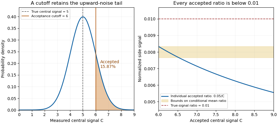
A central-signal cutoff selects upward readout fluctuations and lowers the accepted normalized ratio
. Original Gaussian readout model with true central signal 5, standard deviation 1, cutoff 6 and constant side signal 0.05. Shading marks the accepted tail. The ratio panel shows pointwise accepted ratios and bounds on their conditional mean; it is not measured correlator data. Details.In the historical single-shot correlator, nonlinear mixing encoded delays spatially and an imaging lens recorded the third-harmonic signal on a filtered CCD detector.[ref]
A Single Shot 3rd Order Cross-Correlator for Pulse Contrast and Pulse Shape Measurements by J. Collier and others. Printed pp. 194–195, Description and Figure 2
Selecting a trace by its central pixels conditions subsequent normalization on the same recorded data. Preserve the threshold, background treatment, number attempted and number accepted alongside the shot-resolved pulse-contrast estimator. For independent shots sharing the same acceptance probability, the accepted count has a binomial distribution, carrying information that disappears if only normalized accepted traces are retained.Curvature error in overlap-reference transfer is the residual instrumental correction left when a curved operating-point response is represented by endpoint linear interpolation. Let be the actual log-ratio offset at optical power , and let interpolate its exact values at . Applying as the correction leavesThis deterministic model discrepancy is separate from random uncertainty in the measured endpoints.
The polynomial interpolation error formula gives, for twice continuously differentiable and between the endpoints,for some in that interval. To derive it, subtract a multiple of chosen to make the error vanish also at ; two applications of Rolle's theorem make the second derivative vanish at an intermediate point. If , thenThe maximum product occurs at the midpoint. Halving the reference spacing therefore quarters this worst-case bound when the same curvature bound remains justified.
For an original example, use power in milliwatts, endpoints , , and . The midpoint error is bounded by in log-ratio. The exact functionattains while matching both endpoint corrections perfectly. The corresponding multiplicative error in the corrected optical ratio is . Repeating endpoint measurements indefinitely would reduce their random uncertainty without revealing this midpoint discrepancy.
To guarantee throughout a reference interval under the stated bound, choose spacing satisfyingThe numerical bound and tolerance require spacing no greater than . Outside the endpoint interval, the product error formula needs a curvature bound over the larger range including the extrapolation point; the interior maximum bound cannot simply be reused.
A proposed check measures additional intermediate power settings and repeats at the intended detector bias and beat frequency. It also monitors mode alignment and polarization, which the primary NIST heterodyne apparatus controls separately.[ref]
Frequency response metrology for high-speed optical receivers by Paul D. Hale and others. PDF p.1, Heterodyne measurements, mode matching
Finitely many extra points constrain a response model but do not prove an arbitrary global curvature bound. State how is justified. The GUM's treatment of uncertainty propagation distinguishes local approximations from significant nonlinear effects.[ref]The directional derivative of a clipped logarithmic acquisition time describes the first-order recording extension when several envelope parameters change together at the acquisition threshold. For positive , writeThe logarithmic tail-duration change at the zero-extension boundary article treats a fixed decay time and logarithmic input coordinate. Here consider a boundary point and an additive parameter direction .
The one-sided directional derivative uses positive step sizes:The logarithmic chain rule gives the expression inside the maximum. Differentiating the prefactor contributes zero at the boundary because the clipped logarithm there is zero.
For an original example, let , and . Increase amplitude in direction while decreasing decay time in direction , with . The net fractional direction is , so per unit step. Reversing the direction gives derivative zero, not .
The derivative is positively homogeneous in the direction but is not linear, so no single gradient represents all threshold-crossing perturbations. Above threshold the usual smooth derivative applies; strictly below threshold all sufficiently small changes leave the extension zero. Gaussian input uncertainty at a clipped acquisition-time threshold can consequently produce a mass of outcomes exactly at zero rather than a symmetric distribution around a nominal duration. The directional calculation alone does not assign a confidence level.
This is a conditional optical-envelope calculation. Separating optical power from the receiver's electrical response remains necessary before its parameters describe missed light. NIST independently characterized the detector/cable/oscilloscope response in its pulse calibration procedure.[ref]
Calibration Service for Low-level Pulsed-Laser Radiometers at 1.06 µm: Pulse Energy and Peak Power by Rodney W. Leonhardt. Appendix C.1–C.2, printed pp. 36–37
A derivative can describe parameter sensitivity accurately while the envelope itself still needs experimental justification.The feasible-set boundary in overlap inversion separates joint measurements admitting a finite positive Gaussian radius ratio from measurements incompatible with that forward model. For radius-setting parameter and log-ratio , the admissible region isAt its upper boundary the inferred radius ratio tends to zero; at its lower boundary it becomes arbitrarily large. The joint radius-setting and log-ratio bounds must therefore be checked against the sloping joint boundary, not against a fixed limit evaluated only at the central .
An original ellipsoid calculation gives an exact test for a common joint-set model. Let lie in , with positive definite. For any vector , the maximum of isTo see this, write , , and apply the Cauchy-Schwarz inequality; equality is attained along the corresponding transformed direction.
Use and . The entire ellipse is strictly admissible if both displayed maxima are negative and its smallest is positive. This ellipsoidal admissibility test for overlap data checks every point of the stated joint set. It does not require sampling a coarse grid that might miss the closest approach to the boundary.
For stipulated means , standard-scale parameters , and , the central distance is 0.3. With zero covariance, the upper-boundary excursion isso the ellipse crosses that boundary. With correlation , the covariance is 0.0024 and the excursion becomesThat ellipse stays below the upper boundary; the lower boundary and positive- condition are also satisfied. Correlation changes the geometry even though both marginal uncertainty scales are unchanged.
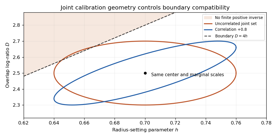
Original joint calibration sets with identical marginal scales: zero correlation crosses the finite-inversion boundary, while correlation +0.8 stays inside
. Details. If a set intersects the forbidden region, report the incompatibility and examine calibration, model adequacy and the meaning of the input bounds. Clipping points and applying the inverse to the survivors changes the propagated set or probability distribution. JCGM 101 separates input assignment, propagation and output summaries and gives conditions for valid Monte Carlo propagation.[ref] An illustrative ellipse is a deterministic set here; interpreting it as a confidence region requires an additional statistical model.
Covariance-consistent rescaling of whitened spectral coordinates changes measurement units or mixes coordinates while transforming their noise model at the same time. If an invertible matrix maps a spectral vector to , thenThe covariance follows directly from the expectation of the transformed error outer product. For positive-definite ,Thus the inverse-covariance inner product, its norms and the resulting whitened angle are invariant. Invariance of noise-whitened spectral angles to the whitening factor establishes the related freedom to rotate the fully whitened coordinates.
For an original example, let , and . Their noise-whitened angle has cosine , or angle about . Converting only the first raw coordinate's numerical units by a factor of 1000 gives and . Using that transformed covariance keeps the cosine exactly .
If the shapes are rescaled but the old covariance is mistakenly retained, the calculated cosine becomes approximately , suggesting an angle only about . A unit conversion would then appear to destroy the separation between signal and nuisance. That apparent change comes from inconsistent uncertainty accounting.
For any full whitening factor , the transformed factor satisfies and gives . The pinned SciPy documentation describes whitening and demonstrates a near-identity covariance after transformation.[ref] Measurement propagation likewise retains all covariance terms under a linear transformation.[ref]
The invertibility condition matters. Noninvertible spectral compression versus a coordinate change can discard information and need not preserve these angles. A transformation estimated from the same noisy observations also brings estimation uncertainty beyond the fixed-matrix identity proved here.
An empty physical confidence set for a detector variance difference occurs when the entire reported interval for the inferred response variance lies below its admissible range. In the nonnegative-profile detector model, . An interval gives a physical width setIt is empty exactly when . The coverage-preserving detector-width bound from a variance interval proves why this intersection and transformation retain the original coverage event.
For an original reading, suppose an explicitly normal measurement model for gives with known standard deviation . The approximately 95 percent interval contains no nonnegative variance. This is disagreement between that interval and the physical model, not a negative physical detector width or an exact measurement of zero width.
Empty sets can occur occasionally even when the model is correct. If and , thenwhere is the standard normal cumulative distribution function. At the physical boundary and , the probability is about ; at it is about . The boundary probability of an empty detector-width confidence set explains why one empty realization is not a logical disproof of the detector model.
Replacing an empty set by the point zero changes the procedure. It must not be presented as though the original interval precisely determined that point. NIST likewise distinguishes an uncertainty interval from an automatically justified confidence level, emphasizing the distributional assumptions behind coverage factors.[ref]
In practice, examine the width estimates, their correlations and the physical convolution assumptions, while retaining the actual negative interval in the measurement record. NIST's short-input receiver-response measurement illustrates how an independently characterized input helps resolve detector broadening.[ref]
Calibration Service for Low-level Pulsed-Laser Radiometers at 1.06 µm: Pulse Energy and Peak Power by Rodney W. Leonhardt. Appendix C.1–C.2, printed pp. 36–37, Figure C1
Neither clipping the estimate nor declaring the response model false follows solely from the sign of one noisy variance difference.The null-space feasibility test for baseline-estimator constraints determines whether any measurement weights can preserve a specified pulse response while removing the requested backgrounds. Write the conditions as . The criterion in constraint redundancy in baseline-noise minimization is that be orthogonal to every vector in the kernel of .
A singular value decomposition makes this a finite test. Let contain an orthonormal basis for the kernel of and the complementary right singular vectors. ThenThe vector is the component of the required responses outside the attainable response space. No covariance weighting can make an exactly infeasible set of responses feasible.
For an original three-reading example, suppose the sampled signal template is constant: . Requiring unit signal response while rejecting a constant baseline gives and . The kernel basis vector has inner product with , so the conditions are incompatible. A constant signal cannot be distinguished from an unknown constant background by those readings alone.
Projecting onto the attainable space gives . The minimum-norm approximate weights are , giving both signal and baseline response one half. Under independent unit-variance errors their variance is only , but this low value belongs to a different, biased measurement response. It does not solve the requested cancellation problem.
A numerical feasibility residual for baseline constraints needs meaningful scaling of the conditions and a justified singular-value tolerance. Changing time units or allowing a small physical leakage changes the numerical interpretation; it must not silently turn an exact rejection requirement into an approximate one.
NIST's before/after pulse baselines motivate the physical need for a separable pulse and background.[ref]
Calibration Service for Low-level Pulsed-Laser Radiometers at 1.06 µm: Pulse Energy and Peak Power by Rodney W. Leonhardt. §3.5, printed p. 8; §7.2, Leakage Effect
Once feasibility is established, minimum-noise weights under baseline moment constraints uses the actual error covariance to choose among valid estimators. Extra timing information or a different signal template can restore identifiability when the original conditions fail.Global orientation ambiguity in a rank-one covariance fit means that covariance identifies an axis without identifying its positive direction. For and ,because . Adding an isotropic transverse-noise term does not remove this equality. The angular resolution set by transverse spectral noise can make each local orientation lobe narrow while leaving the two directed orientations indistinguishable.
For an original example, let and . Both and giveThe eigenvalues are four and zero, and the principal eigenvector can be written as either or its negative. More samples can improve estimation of this matrix without choosing between those signs.
In a zero-mean Gaussian covariance model, equal covariance gives equal probability laws, including the supported line in the singular case.[ref]
SciPy 1.16.2 documentation. scipy.stats.multivariate_normal, mean/cov parameters and Notes on singular covariance
No fitting procedure using only that law can distinguish the two parameter labels. A fitting range removes duplicate labels by convention; it does not measure the sign of a physical direction.For example, local high-likelihood neighborhoods around and may each span only a few degrees. Reporting only the first as uncertainty in a directed angle discards an equally supported region unless additional information rules it out. A prior or coordinate convention that selects one sign should be distinguished from an experimental observation.
Sign-sensitive measurements that resolve a covariance-axis ambiguity can supply information outside the covariance-only model, such as an independently calibrated signed mean or phase reference. If the scientific quantity is genuinely an unoriented axis, an angle modulo is already the appropriate parameter. The interpretation of the parameter determines whether the ambiguity needs resolving.
A validated lower bound on a power-law tail exponent is an exponent constraint that is justified over the future interval where it is used to bound unrecorded energy. A fitted slope over a finite observation window is not by itself such a guarantee. Acquisition duration from a power-law tail-energy tolerance needs a global optical-power envelope, including a lower exponent limit above one for its finite-energy guarantee.
One sufficient condition, for positive absolutely continuous power, isIntegrating the logarithmic derivative gives . The time-dependent decay-rate envelope provides the equivalent integrating-factor argument when zeros of the power need handling. This is a sufficient condition, not a necessary characterization of every bounded tail.
For an original conditional estimation example, assume an exact power-law family with known and initial power . At , a measured ratio range yieldsapproximately . Within that assumed family, the lower endpoint gives a conservative extension about for a remaining-energy tolerance. A nominal exponent two would instead require .
The ratio interval constrains the exponent only conditional on the exact family, known time scale and suitable measurement uncertainty. It cannot exclude a later secondary pulse or a transition to a slower law after the observed window. Future-domain validity of a fitted power-law optical envelope therefore requires independent physical justification or explicitly limited claims. If the justified exponent set reaches one, this envelope alone supplies no finite all-time energy guarantee.
Finally, the measured trace must represent optical power rather than an uncorrected receiver tail. NIST measured the detector, cable and oscilloscope together using a short characterized optical input before correcting pulse measurements.[ref]
Calibration Service for Low-level Pulsed-Laser Radiometers at 1.06 µm: Pulse Energy and Peak Power by Rodney W. Leonhardt. Appendix C.1–C.2, printed pp. 36–37, Figure C1 and response-measurement procedure
The exponent example is an original model calculation, not an observed law attributed to that apparatus.The rifleman, Acanthisitta chloris, is a small New Zealand forest bird in Acanthisittidae. It has short wings, a very short tail and a slender, slightly upturned bill. Males and females differ in plumage: males have green upperparts, while females are more brown and speckled, an example of sexual dimorphism.[ref]
Rifleman in New Zealand Birds Online. Identification
Its way of feeding is closely tied to the forest's surfaces. A rifleman searches tree trunks, bark and foliage for small invertebrates and usually moves between feeding sites by short flights. Watching whether a bird probes beneath bark, picks prey from a leaf or catches it in the air distinguishes different foraging actions rather than treating all insect eating as the same behavior.[ref]
The species also illustrates cooperative breeding. Related young can help feed a later brood alongside the breeding pair. To describe this correctly, an observer must identify individuals and record who delivers food: counting visits to a nest alone cannot distinguish parental care from help supplied by other group members. Such observations connect the family group to the survival of young without assuming that every bird at a nest is a parent.[ref]
Rifleman in New Zealand Birds Online. Breeding: helpers feed nestlings; both sexes provide parental care
Angular resolution set by transverse spectral noise quantifies how sharply an observed spectral vector constrains the orientation of an anisotropic two-coordinate noise model. Use the covariance from transverse-noise limit of a rotating rank-one covariance model, with known longitudinal standard deviation and transverse standard deviation . For an observation of length aligned with orientation , the Gaussian density givesThe determinant is independent of orientation, so the angular dependence comes entirely from the covariance-weighted residual.[ref]
SciPy 1.16.2 documentation. scipy.stats.multivariate_normal, Notes, full-rank Gaussian density
Define a local half-width by a chosen log-density drop . For , the lobe around has half-widthWhen this angle is small and , it is approximately . If , even an orthogonal orientation fails to reach that drop, so this local-width criterion does not exclude any orientation. At or equal noise scales, the observation has no angular preference in this model.
For an original example, choose , and in consistent signal units. Then . A drop gives half-width about radians, or . Reducing only the transverse standard deviation to approximately halves the width. Increasing a numerical regularization parameter is not an experimental improvement in this noise scale.
The global orientation ambiguity in a rank-one covariance fit remains: orientations separated by give the same covariance. A narrow local lobe does not distinguish those two orientations. Nor is a fixed log-density drop automatically a confidence interval with a stated coverage probability. Multiple observations, unknown noise scales and experimental nuisance parameters require their corresponding inference model.
Repeated reference spectra under stable conditions can estimate the longitudinal and transverse noise components. Their covariance must include shared calibration effects, as required by the measurement-propagation rule.[ref]
Guidelines for Evaluating and Expressing the Uncertainty of NIST Measurement Results by Barry N. Taylor and Chris E. Kuyatt. Appendix A, equation A-3
The numerical example is a model calculation in spectral coordinates, rather than a specification of a particular optical instrument.The conditioning of tie-line phase-fraction inference describes how strongly composition perturbations change an inferred phase fraction. For a binary mixture with distinct endpoints, the lever rule gives . Its absolute sensitivity to , with endpoints fixed, is . This is an absolute amplification coefficient; a relative condition number additionally depends on the chosen input and output scales.
For an interior , the differential in tie-line phase-fraction sensitivity yieldsto first order. If each composition perturbation is bounded by , this becomes . For original stipulated , endpoint separations and give local worst-case bounds and . Tenfold closer endpoints make the same composition precision tenfold less informative about phase amount. Correlations can change the attainable combinations of errors, as common affine calibration cancellation in the lever rule illustrates.
For fixed multicomponent endpoints and overall-composition covariance matrix , the tie-line phase-fraction uncertainty isThe denominator is endpoint separation after a whitening transformation: separation must be compared with measurement precision, not only plotted distance. This follows from covariance-based uncertainty propagation and the linear fit.[ref]
Guide to the expression of uncertainty in measurement by JCGM. §§5.1–5.2, sensitivity coefficients and covariance propagation
Near coincident endpoints the inverse problem becomes poorly informative, and at coincidence it is undefined. Near the physical bounds, a large propagated uncertainty also warns that the interior linear approximation may fail. More numerical digits in the fitted answer do not resolve this measurement limitation.
The residual correction in tie-line sensitivity accounts for rotation of a fitted liquid-liquid tie line when the measured overall composition does not lie exactly on it. In independent mole fraction coordinates, set , hold a symmetric positive-definite matrix fixed, and use the interior unconstrained tie-line phase-fraction fit. With , residual , and row vectors , , its differential isThe full derivation is in tie-line phase-fraction sensitivity. The normal equation makes orthogonal to in the chosen metric; it does not make the residual zero.
For an original example, take , , and . The third mole fraction is fixed by closure. These choices giveIncreasing only the first coordinate of by predicts a phase fraction change . Omitting the correction misses the second contribution even though the fit satisfies its normal equation. A centered finite-difference recalculation as the perturbation shrinks tests this derivative directly.
This is a local sensitivity, not an uncertainty until combined with the joint input covariance matrix.[ref]
Guide to the expression of uncertainty in measurement by JCGM. §§5.1.3–5.1.4, sensitivity coefficients; §5.2.2, correlated-input propagation
The formula assumes distinct endpoints and an interior fit with fixed . A changing metric requires sensitivity of a tie-line fit to its weight matrix; a constrained boundary requires a separate local analysis. A nonzero residual can reflect composition noise or model mismatch and does not independently establish liquid-liquid equilibrium.Common affine calibration cancellation in the lever rule is the exact invariance of the binary mixture phase fraction under the same affine map applied to the overall composition and both endpoints. For ,Both a shared offset and a shared scale cancel. The map must be common to all three measurements; separately fitted calibration curves or sample-dependent effects do not satisfy that assumption.
An original example has , , and . Applying gives measured values , and , still yielding . If only the overall-composition reading then receives an additional error, its inferred fraction changes by . Common calibration cancellation leaves independent sample errors intact.
The covariance matrix formulation explains why treating the shared errors as independent gives a false uncertainty. In input order , the Jacobian matrix row isIt annihilates both the common-offset direction and the common-scale direction , since . A joint covariance matrix representing only these shared affine influences therefore gives . The measurement guide explicitly identifies common instruments and reference data as sources of correlation that must be retained.[ref]
Guide to the expression of uncertainty in measurement by JCGM. §5.2.2, equation13; §5.2.4, common influences
Analyzing the overall sample and separated phases under one unchanged instrument calibration can realize this common contribution; repeating only one sample under another calibration breaks it. The cancellation is a property of this binary ratio. It does not remove nonlinear response, composition closure errors, endpoint misidentification or uncertainty in whether the samples establish liquid-liquid equilibrium.
Pulse-contrast ratio denominator noise is the distortion introduced when a noisy central pulse signal is used to normalize a side-delay signal. A shot-resolved pulse-contrast estimator uses after background correction, so errors in affect both precision and the distribution of the ratio.
For central values with , a second-order local expansion givesThis approximation requires sufficiently small fluctuations and well-behaved ratio moments. It shows why an unbiased central-signal measurement need not give an unbiased normalized ratio. First-order uncertainty propagation alone describes local spread, not this mean shift; the GUM warns that nonlinear models can require higher-order terms.[ref]
Guide to the expression of uncertainty in measurement by JCGM. §5.1.2, nonlinear functions; §5.2, correlated inputs
An original bounded example takes constant side signal and equally likely central readings or 11. The mean central reading is 10, so the ratio of means is 0.01. ButThe second-order prediction is 0.0101 because . Increasing the number of such shots estimates the shifted mean more precisely; it does not remove the nonlinear effect.
Correlation can instead make normalization exact. If for every accepted shot with nonzero , their ratio is always , however variable the common multiplier. This is a different error structure from adding independent noise to the two channels. A shared additive background is also not generally equivalent to a shared multiplicative gain.
Near zero, even existence of a mean can fail. If is fixed and is uniform on , every ratio is positive butThis mathematical example explains why “the denominator was never exactly zero” is insufficient. Detector noise is not asserted to follow this distribution.
A pulse-contrast denominator acceptance rule such as changes the sampled population. Report the rule, rejected-shot count and dependence between brightness and pulse shape. The primary single-shot correlator's nonlinear gate and CCD readout motivate acquiring the relevant signals together, but do not guarantee that all ratios are statistically well conditioned.[ref]
A Single Shot 3rd Order Cross-Correlator for Pulse Contrast and Pulse Shape Measurements by J. Collier and others. printed pp. 194–195, Description and Fig. 2
Resolve the denominator and background experimentally before interpreting a long average of ratios.Reference-versus-sample allocation in repeated isotope-ratio measurements distributes a finite measurement budget between sample readings and the reference used to calibrate them. Suppose independent sample and reference readings have first-order gain-error variances and . Averaging sample readings and reference readings gives log stiffness-ratio variancewhere is the variance of a differential calibration error shared by all ratio estimates. The shared-reference floor in averaged isotope stiffness ratios explains why that last component does not average down. Covariance propagation must reflect which observations and calibration influences are actually shared.[ref]
Let one sample reading cost budget units and one reference reading cost , with . Treating counts continuously for the initial optimization, a constraint multiplier givesThe counts are proportional to standard uncertainty divided by the square root of cost, rather than simply to each variance. A budget-independent common component changes the attainable floor but not this optimum ratio under the stated model.
For an original example, take equal costs, , and 40 total readings. The optimum is 30 sample and ten reference readings. Without a common component, the predicted log-ratio standard uncertainty is about , compared with for twenty of each. A common standard uncertainty raises those values to about and , respectively.
An integer allocation near a continuous isotope-reference optimum must compare feasible neighboring count choices and any acquisition-order constraints. More reference readings help only to the extent that their errors are independent; repeatedly measuring an unchanged unknown calibration bias does not create independent references. If reference drift depends on elapsed time, a single constant cost and common-variance term may be inadequate.
In practice, record which reference observations calibrate which sample spectra and account for any correlated peak fitting, isotope-composition uncertainty and spectral offsets. The variance and cost model above is a chosen allocation problem, not an experimentally established precision specification for an isotope measurement system.
Pinned article: Introduction to the OurBigBook Project
Welcome to the OurBigBook Project! Our goal is to create the perfect publishing platform for STEM subjects, and get university-level students to write the best free STEM tutorials ever.
Everyone is welcome to create an account and play with the site: ourbigbook.com/go/register. We belive that students themselves can write amazing tutorials, but teachers are welcome too. You can write about anything you want, it doesn't have to be STEM or even educational. Silly test content is very welcome and you won't be penalized in any way. Just keep it legal!
Intro to OurBigBook
. Source. We have two killer features:
- topics: topics group articles by different users with the same title, e.g. here is the topic for the "Fundamental Theorem of Calculus" ourbigbook.com/go/topic/fundamental-theorem-of-calculusArticles of different users are sorted by upvote within each article page. This feature is a bit like:
- a Wikipedia where each user can have their own version of each article
- a Q&A website like Stack Overflow, where multiple people can give their views on a given topic, and the best ones are sorted by upvote. Except you don't need to wait for someone to ask first, and any topic goes, no matter how narrow or broad
This feature makes it possible for readers to find better explanations of any topic created by other writers. And it allows writers to create an explanation in a place that readers might actually find it.
Figure 1. Screenshot of the "Derivative" topic page. View it live at: ourbigbook.com/go/topic/derivativeVideo 2. OurBigBook Web topics demo. Source. - local editing: you can store all your personal knowledge base content locally in a plaintext markup format that can be edited locally and published either:This way you can be sure that even if OurBigBook.com were to go down one day (which we have no plans to do as it is quite cheap to host!), your content will still be perfectly readable as a static site.
- to OurBigBook.com to get awesome multi-user features like topics and likes
- as HTML files to a static website, which you can host yourself for free on many external providers like GitHub Pages, and remain in full control

Figure 2. You can publish local OurBigBook lightweight markup files to either OurBigBook.com or as a static website.
Figure 3. Visual Studio Code extension installation.
Figure 5. . You can also edit articles on the Web editor without installing anything locally. Video 3. Edit locally and publish demo. Source. This shows editing OurBigBook Markup and publishing it using the Visual Studio Code extension. 
- Infinitely deep tables of contents:




All our software is open source and hosted at: github.com/ourbigbook/ourbigbook
Further documentation can be found at: docs.ourbigbook.com
Feel free to reach our to us for any help or suggestions: docs.ourbigbook.com/#contact